Introduction

Source detection in Poisson-count photon imaging is commonly carried out by fitting a parametric source model on top of a known background and summarizing the result by a likelihood-ratio statistic. Under the standard Cash-statistic formulation , the natural statistical object is the Cash improvement $\Delta C = C_\mathrm{null} - C_\mathrm{best}$, with $C$ proportional to twice the negative Poisson log-likelihood. Detection pipelines typically report a monotone transform of $\Delta C$ as a “detection likelihood”; in the XMM-Newton Science Analysis System, for example, emldetect fits a three-parameter source model (one free amplitude and two free position coordinates) to Poisson-count images and reports $\mathrm{DET\_ML}$, an incomplete-gamma transform of the underlying $\Delta C$. The reported detection-likelihood statistic is operationally important: it is used to decide which sources enter a catalog, to define detection thresholds, and to construct sensitivity maps.

Sensitivity maps and source counting methodologies have been extensively developed and applied in major X-ray surveys . The statistical treatment of Poisson source detection, limits, and likelihood ratio methods also has a long history in high-energy astrophysics . The emldetect tool has been the standard for the XMM-Newton serendipitous survey catalogs .

We emphasize at the outset that $\mathrm{DET\_ML}$ is used throughout this paper strictly as an operational monotonic threshold scale inherited from the SAS convention. We do not interpret it as a calibrated frequentist false-alarm probability. The standard $\chi^2_3$ null distribution underlying the incomplete-gamma transform assumes interior regularity conditions that are violated at the boundary of the parameter space ($S=0$) and when position parameters are unidentifiable under the null. More generally, the distribution of the Cash statistic itself departs from its high-count $\chi^2$ limit in the low-count Poisson regime . Our use of the $\mathrm{DET\_ML}$–$\Delta C$ conversion is therefore purely operational: it maps a detection threshold chosen by the survey analyst into the corresponding $\Delta C$ value, where the observable-conditioned theory applies.

The practical threshold regime is low signal. For many XMM-Newton applications the relevant sensitivity-map range is $\mathrm{DET\_ML}$ of order 6–10. This is the regime where source counts are steep, Poisson fluctuations matter, and a small shift in the detection threshold can change the inferred limiting flux. It is therefore also the regime where Eddington bias becomes important: random upward fluctuations are preferentially selected near the detection boundary, and the selected sample no longer represents the untruncated parent distribution .

The core challenge is not the absence of a predictable mean. The expected $\Delta C$ at a fitted source has long been computed analytically and used as a single deterministic value in X-ray sensitivity-map construction. Within the SAS itself, esensmap carries an emldetect-style analytical Cash-statistic model from version 4.0 onward, following the emldetect $\Delta C$ formalism of the 3XMM and 4XMM catalogue pipelines ; outside it, the same expectation evaluated at the detected (rather than the injected) source flux was used to construct the sensitivity map of the New-ANGELS XMM legacy survey . What this prior literature has not done is treat $\Delta C$ as a sample from a non-trivial sampling distribution.

Yet the distributional moments are inputs that any systematic treatment of Eddington bias or flux-limit precision must eventually incorporate. While this work does not construct a full Eddington-bias kernel, characterizing the conditional mean and variance of $\Delta C$ is a necessary foundational step. We provide an analytic backbone (the conditional mean and Fisher-projected variance of $\Delta C$ as explicit pixel-sum formulae) that reduces the complex threshold calibration problem to interpolating a slowly-varying scalar residual in detector-position space. The theory itself closes in the high-signal regime; in the threshold band where $\mathrm{DET\_ML}=6$–10, an empirical residual calibration absorbs the beyond-Fisher bias and the implementation-dependent offset of standalone emldetect. The pipeline-reported detection-likelihood statistic, however, is a nonlinear incomplete-gamma transform of $\Delta C$ and is therefore not Gaussian; cuts on the reported statistic near the detection threshold truncate a non-Gaussian distribution selectively, which is exactly the regime in which sensitivity maps and source-count corrections are most vulnerable to Eddington bias.

The paper is organized around the following narrative. Section 2 establishes the observable-conditioning principle. Section 3 derives the three-parameter $\Delta C$ theory as explicit pixel-sum formulae. Section 4 validates the theory against self-consistent reference-fitter simulations, confirming high-signal closure and characterizing the low-signal bias. Section 5 constructs the empirical residual calibration required by standalone emldetect in the threshold band. Section 6 describes two catalog applications of the calibrated $\Delta C$ distribution: interpreting traditional $\mathrm{DET\_ML}$-selected catalogs and constructing fitted-amplitude percentile sensitivity maps. Section 7 catalogs the validated and unvalidated domains. Section 8 summarizes the conclusions.

Observable-Conditioned Residuals

The central statistical object is the conditional expectation of $\Delta C$ in observable space,

$$E[\Delta C | \widehat{S}, b, \mathrm{psf}, \mathrm{mask}],$$

where $\widehat{S}$ is the fitted source amplitude, $b$ is the local background in counts per pixel, $\mathrm{psf}$ is the pixelized PSF template used by the fitting model, and $\mathrm{mask}$ is the image region included in the fit. Section 3 derives this expectation analytically; Section 5 turns it into the operational standalone-emldetect threshold calibration, and Section 6 into two catalog-level uses: a backward interpretation of traditional $\mathrm{DET\_ML}$ selection and a forward construction of fitted-amplitude threshold-crossing cuts.

Conditioning on fitted amplitude

In a simulation the injected source strength $S_\mathrm{true}$ is known and gives cleaner diagnostic plots than $\widehat{S}$, but it is not a usable conditioning variable for a detection theory: $S_\mathrm{true}$ is absent from every real image and from every emldetect source table, and is unavailable when building a sensitivity map. A theory conditioned on $S_\mathrm{true}$ cannot be applied to real detections or to fake-source recovery tests without injecting information that is not present in the use case. Throughout, $S_\mathrm{true}$ denotes a simulation-generation label only, and $\widehat{S}$ is the conditioning variable. A result conditioned on $S_\mathrm{true}$ tests whether the model behaves sensibly for a known injected flux; a result conditioned on $\widehat{S}$ tests whether it can be used after a detection has been fit. Only the latter is relevant for standalone-emldetect sensitivity-map work.

Residual decomposition

For each source or fake-source trial the theory prediction is evaluated at the observed fitted quantities,

$$\mu_{3p,i} = E_{\mathrm{theory}}[\Delta C | \widehat{S}_i, b_{i}, \mathrm{psf}_i, \mathrm{mask}_i],$$

and the residual is

$$R_{i} = \Delta C_{i} - \mu_{3p,i}$$

For a sample or bin,

$$\begin{aligned} \langle \Delta C \rangle &= \langle R \rangle + \langle \mu_{3p} \rangle, \\ \mathrm{Var}(\Delta C) &= \mathrm{Var}(R) + \mathrm{Var}(\mu_{3p}) + 2\,\mathrm{Cov}(R, \mu_{3p}) \end{aligned}$$

Only when $\mu_{3p}$ is approximately constant across the bin does the observed $\Delta C$ width reduce to $\mathrm{Var}(R)$; mixed-$\widehat{S}$ or mixed-position samples otherwise introduce apparent variance effects that are not properties of the conditional theory. Properly conditioned in $\widehat{S}$ bins, $\sigma^2_{3p}$ is accurate to within ${\sim}7$% across the full $0$–$14'$ off-axis range, with a mild low-$\widehat{S}$ overestimate and no resolved off-axis dependence; the corresponding global correction is given in Section 4.3 (Equation [eq:sigma-corr]). Earlier single-$S_\mathrm{true}$ binning instead mixes $\widehat{S}$ within each bin and inflates the apparent off-axis scatter, an artifact of the conditioning variable rather than a property of the theory.

Threshold selection in $\Delta C$ space

$\mathrm{DET\_ML}$ is a nonlinear monotone tail-probability transform of $\Delta C$,

$$\mathrm{DET\_ML}= -\ln Q(\nu/2, \Delta C/2),$$

with $\nu=3$ and $\mathrm{shape}=1.5$ for the single-source three-parameter fit. The corresponding inverse is $$\Delta C_{\mathrm{th}} = 2\,Q_x^{-1}(1.5, \exp(-\mathrm{DET\_ML})), \label{eq:detml-inverse}$$ where $Q$ is the regularized upper incomplete gamma function and $Q_x^{-1}$ denotes inversion with respect to its second argument. Thus $\mathrm{DET\_ML}=6,\,8,\,10$ correspond to $\Delta C_{\mathrm{th}}=14.3,\,18.6,\,22.8$, respectively. A Gaussian residual in $\Delta C$ is therefore not Gaussian in $\mathrm{DET\_ML}$, and selecting on observed $\mathrm{DET\_ML}$ is a selection on the same noisy quantity whose distribution is being measured: it truncates the residual distribution and biases its mean upward near the threshold. Threshold ranges are accordingly translated into $\Delta C$ using the three-parameter convention and applied as theoretical or predicted $\Delta C$ conditions (such as $\mu_{3p,\rm ref}\in[\Delta C_\mathrm{ML6},\Delta C_\mathrm{ML10}]$) or as $\widehat{S}$ bins whose typical predicted $\Delta C$ lies in that interval. This keeps the conditioning independent of the observed stochastic fluctuation in $\Delta C_\mathrm{eml}$.

Three-Parameter $\Delta C$ Theory

While the underlying statistical framework (based on the Kullback–Leibler divergence for the conditional mean and the Cramér–Rao delta-method under Wilks’ theorem for the variance) is standard likelihood theory, the novelty here is its specific evaluation on a 2D pixelized Poisson X-ray dataset. The Fisher-matrix structure is closely related to Cramér–Rao analyses of joint astrometry and photometry for pixel-array point-source measurements . The conditional mean and approximate variance of $\Delta C$ for the standard single-source PSF fit, with one free amplitude and two free position coordinates, are derived below as explicit pixel-sum formulae.

Pixelized Poisson model

Consider a fitting region containing pixels indexed by $i$. The observed counts are independent Poisson random variables,

$$Y_{i} \sim \mathrm{Poisson}(\mu_i)$$

For a single source on a locally known background, the fitted source model is

$$\begin{aligned} \mu_i(\theta) &= b_{i} + S\, p_{i}(x, y), \\ \theta &= (S, x, y) \end{aligned}$$

Here $b_i$ is the background expectation in pixel $i$, $S$ is the source amplitude in the same units used by the image model, and $p_i(x,y)$ is the pixelized PSF template shifted to position $(x,y)$. The PSF is normalized over the full template grid, $\sum_i p_i=1$; the mask $M_i$ then selects the fitting footprint. Thus $S$ denotes the total source amplitude in the template convention, not the counts enclosed by the fitting mask. In the current PN band-4 validation runs, $b_i$ is usually a constant $b$ inside the fitting region, but the notation allows the background to vary by pixel.

A binary fitting mask $M_i$ selects the pixels included in the fit; the primary results in this paper use binary masks. A weighted-mask extension exists for fractional weights, but when the weights are exactly 0 or 1 the weighted formula reduces to the binary-mask convention used here.

Cash statistic and $\Delta C$ sign convention

Ignoring constants independent of the model parameters, the Cash statistic is

$$C(\theta) = 2 \sum_i M_{i} \bigl[\mu_i(\theta) - Y_{i} \ln \mu_i(\theta)\bigr]$$

The null model is the background-only model, $\mu_{i,0} = b_{i}$. The likelihood-ratio Cash improvement is

$$\Delta C = C_{\mathrm{null}} - C_{\mathrm{best}}$$

With this sign convention, a better source fit gives positive $\Delta C$. At a fixed fitted model $\mu_i$, the statistic can be written as

$$\Delta C = 2 \sum_i M_{i} \bigl[ b_{i} - \mu_i + Y_{i} \log(\mu_i / b_{i}) \bigr]$$

Conditional mean at fixed fitted result

The observable-conditioned theory evaluates the moments at the fitted result

$$\begin{aligned} \widehat{\theta} &= (\widehat{S}, \widehat{x}, \widehat{y}), \\ \mu_i &= b_{i} + \widehat{S}\, p_{i}(\widehat{x},\widehat{y}) \end{aligned}$$

The Asimov image for this fitted model is $Y_i = \mu_i$. Substituting this into the Cash improvement gives the conditional mean

$$\mu_{3p}(\widehat{S},b,\mathrm{psf},\mathrm{mask}) = 2\sum_i M_i\left[\mu_i\ln\left(\frac{\mu_i}{b_i}\right)-(\mu_i-b_i)\right] \label{eq:mu3p}$$

For a constant background $b_i = b$ and normalized PSF $p_i$, this becomes the explicit pixel sum: $$\mu_{3p} = 2 \sum_i M_{i} \bigl[ (b + \widehat{S}\, p_{i}) \log\bigl((b + \widehat{S}\, p_{i})/b\bigr) - \widehat{S}\, p_{i} \bigr] \label{eq:mu3p-pixel-sum}$$

This mean depends on the pixelized PSF and the mask through the full pixel sum. It is not a function only of a Gaussian width or of low-order PSF moments, although such summaries can be useful diagnostics.

Writing $r_i = \mu_i / b_i$, Eq. [eq:mu3p] becomes $\mu_{3p} = 2\sum_i M_i b_i [r_i \ln r_i - (r_i - 1)]$, which is the per-pixel Poisson Kullback–Leibler divergence from background to source-plus-background, summed over the fitting region. This is precisely the non-centrality parameter of the asymptotic non-central $\chi^2_3$ distribution for the likelihood ratio . The convexity of $r\ln r - (r-1)$ guarantees $\mu_{3p} \ge 0$.

An important asymmetry exists between the mean and the variance derived below. The mean $\mu_{3p}$ is a zeroth-order Asimov quantity: it substitutes the expected counts $Y_i = \mu_i$ into the Cash improvement but does not account for the absorption of Poisson fluctuations by the fitted parameters (the look-elsewhere effect from position optimization). The variance $\sigma^2_{3p}$, by contrast, already includes a first-order correction for this absorption via the Fisher projection of Section 3.6. This asymmetry is the origin of the positive beyond-Fisher bias observed at low fitted signal (Section 4.3): position parameters can migrate to absorb a local Poisson upward fluctuation, inflating $\Delta C$ beyond the Asimov prediction. The empirical residual $R_\mathrm{eml}$ introduced in Section 5.1 absorbs this effect into an operational calibration.

Linearized score constraints

The best-fit parameters satisfy the score equations. For any fitted parameter $\theta_a \in \{S, x, y\}$,

$$dC/d\theta_a = 0$$

Linearizing around the fitted model, write

$$\begin{aligned} Y_{i} &= \mu_i + \eta_i, \\ E[\eta_i] &= 0, \\ \mathrm{Var}(\eta_i) &= \mu_i \end{aligned}$$

The first-order score constraint is

$$\sum_i M_{i} (d\mu_i/d\theta_a)\, \eta_i / \mu_i = 0$$

There are three such constraints:

$$\begin{aligned} d\mu_i/dS &= p_{i}, \\ d\mu_i/dx &= \widehat{S}\, dp_i/dx, \\ d\mu_i/dy &= \widehat{S}\, dp_i/dy \end{aligned}$$

These constraints are the reason a three-parameter fit is not equivalent to a simple unconstrained Poisson sum. Fluctuations along the fitted amplitude and position directions are absorbed by the fit and must be projected out when computing the residual variance.

$\Delta C$ residual variance before projection

At fixed fitted model, the first-order stochastic part of $\Delta C$ is

$$R_{\mathrm{linear}} = 2 \sum_i M_{i}\, \eta_i \log(\mu_i / b_{i})$$

If the fitted parameters were not constrained by the score equations, the variance of this linear residual would be

$$\sigma^2_\mathrm{unc} = 4 \sum_i M_{i}\, \mu_i \ln^2\!\left(\frac{\mu_i}{b_{i}}\right)$$

This term, $\sigma^2_\mathrm{unc}$, is useful as a diagnostic but is not the final variance formula for the fitted likelihood ratio. It ignores the fact that $S$, $x$, and $y$ were chosen to maximize the likelihood. Because the Fisher projection below subtracts a positive semidefinite quadratic form, $\sigma^2_\mathrm{unc}$ is an upper bound on the projected variance within the local Gaussian approximation.

Fisher projection for three fitted parameters

Define the Fisher information matrix for the three fitted parameters:

$$I_{ab} = \sum_i M_{i} (d\mu_i/d\theta_a)(d\mu_i/d\theta_b) / \mu_i$$

For $\theta = (S,x,y)$, the entries are

$$\begin{aligned} I_{SS} &= \sum_i M_{i}\, p_{i}^2 / \mu_i \\ I_{Sx} &= \sum_i M_{i}\, \widehat{S}\, p_{i} (dp_i/dx) / \mu_i \\ I_{Sy} &= \sum_i M_{i}\, \widehat{S}\, p_{i} (dp_i/dy) / \mu_i \\ I_{xx} &= \sum_i M_{i}\, \widehat{S}^2 (dp_i/dx)^2 / \mu_i \\ I_{xy} &= \sum_i M_{i}\, \widehat{S}^2 (dp_i/dx)(dp_i/dy) / \mu_i \\ I_{yy} &= \sum_i M_{i}\, \widehat{S}^2 (dp_i/dy)^2 / \mu_i \end{aligned}$$

The covariance between the $\Delta C$ residual and the score direction $\theta_a$ is encoded by

$$g_{a} = \sum_i M_{i} \log(\mu_i/b_{i})\, (d\mu_i/d\theta_a)$$

Explicitly,

$$\begin{aligned} g_{S} &= \sum_i M_{i}\, p_{i} \log(\mu_i/b_{i}) \\ g_{x} &= \sum_i M_{i}\, \widehat{S}\, (dp_i/dx) \log(\mu_i/b_{i}) \\ g_{y} &= \sum_i M_{i}\, \widehat{S}\, (dp_i/dy) \log(\mu_i/b_{i}) \end{aligned}$$

Under the Gaussian/Fisher approximation, conditioning on the fitted score constraints subtracts the projection of the residual onto the fitted parameter subspace. This is the standard multivariate Gaussian conditional-variance identity, $$\mathrm{Var}(R\mid U=0)=\mathrm{Var}(R) -\mathrm{Cov}(R,U)\,\mathrm{Var}(U)^{-1}\,\mathrm{Cov}(U,R),$$ where $U$ denotes the vector of linearized score constraints. The resulting variance is

$$\sigma^2_{3p} = 4\left[\sum_i M_i\mu_i\ln^2\left(\frac{\mu_i}{b_i}\right) - g^T I^{-1}g\right] \label{eq:var3p}$$

The projection $g^T I^{-1}g$ can be computed conveniently via the block structure of the Fisher matrix. Writing $$I = \begin{pmatrix} I_{SS} & H \\ H^T & K \end{pmatrix}, \label{eq:block-inverse-I}$$ where $H$ contains the $S$-position cross terms and $K$ is the $2\times2$ position block for $x$ and $y$, the projection becomes $$\begin{split} g^T I^{-1} g =&\; (g_{S} - H K^{-1} g_\mathrm{pos})^2 / (I_{SS} - H K^{-1} H^T) \\ &+ g_\mathrm{pos}^T K^{-1} g_\mathrm{pos}, \end{split} \label{eq:block-inverse-result}$$ where $g_\mathrm{pos} = (g_x, g_y)^T$. This block form makes the position projection explicit and is numerically convenient for a large grid of $\widehat{S}$ and $b$ values. If the position directions are removed and only $S$ is fit, the formula reduces to the amplitude-only one-parameter expression.

Validity range of the variance approximation

The variance expression $\sigma^2_{3p}$ is a local Gaussian/Fisher approximation around the fitted model. It is expected to be accurate when the likelihood surface is close to quadratic and when the fitted source is strong enough that position optimization does not absorb isolated Poisson noise features. The properly $\widehat{S}$-conditioned variance diagnostic, and the global low-$\widehat{S}$ correction that absorbs the residual deficit, are presented in Section 4.3 and Figure [fig:deltac-scatter-variance]. These Fisher/Wilks approximations fail at the $S=0$ boundary and become incomplete in the low-signal threshold band; the remaining threshold-band residual is therefore handled empirically in Section 5.

Self-Consistent Reference-Fitter Validation

The reference fitter is not intended to be a reimplementation or replacement of SAS emldetect. Instead, it provides a controlled matched-model baseline: the simulated sources, the Poisson likelihood fitter, and the theoretical moment calculation all use the same psfgen PSF template, fitting footprint, and likelihood convention. This construction separates two questions that are otherwise entangled in the standalone pipeline comparison. First, it tests whether the analytic observable-conditioned $\Delta C$ mean and Fisher-projected variance close when the data-generating model, fitting model, and theory are matched. Second, by comparing standalone emldetect against this controlled baseline, we can identify the remaining discrepancy as a combination of low-signal asymptotic bias and pipeline-specific implementation residuals (optimizer behavior, PSF sampling, numerical discretization, and mask conventions). The empirical $R_\mathrm{eml}$ calibration in Section 5 is designed to absorb this latter residual in the operational threshold band.

Simulation design

The reference validation uses high-statistics simulations for the XMM-Newton PN band-4 configuration, spanning 17 detector positions, eight injected source strengths, six background levels, and 1000 realizations per grid cell. This yields 816,000 simulated fits; after requiring normal optimizer convergence and fitted amplitudes $0 < \widehat{S} < 500$, 811,194 fits remain.

The simulations use XMM-Newton SAS v20.0.0, a standard $\mathtt{ecut}=15$ extraction footprint, and a robust Nelder–Mead reference fitter. No detector position is removed from the reference-fitter validation. The standalone calibration grid in Section 5 excludes an edge-affected calibration position whose local PSF geometry violates the stationary-background assumption used by the empirical residual model. For standalone comparisons, the empirical statistic is extracted directly from the catalog $\mathrm{DET\_ML}$ column and converted using $\Delta C_\mathrm{eml} = 2\,Q_x^{-1}(1.5,\exp(-\mathrm{DET\_ML}))$ with $\nu=3$.

Each simulated source is fit with a three-parameter Poisson likelihood fitter. For every row, the theory is evaluated at the fitted source strength:

$$\begin{aligned} \mu_{3p} &= E[\Delta C | \widehat{S}, b, \mathrm{psf}, \mathrm{mask}], \\ \sigma^2_{3p} &= \mathrm{Var}[\Delta C | \widehat{S}, b, \mathrm{psf}, \mathrm{mask}] \end{aligned}$$

The diagnostic residual is

$$Z = (\Delta C_{\mathrm{obs}} - \mu_{3p}) / \sqrt{\sigma^2_{3p}}$$

This is an observable-conditioned validation because the prediction uses the fitted amplitude $\widehat{S}$, not the injected amplitude $S_\mathrm{true}$.

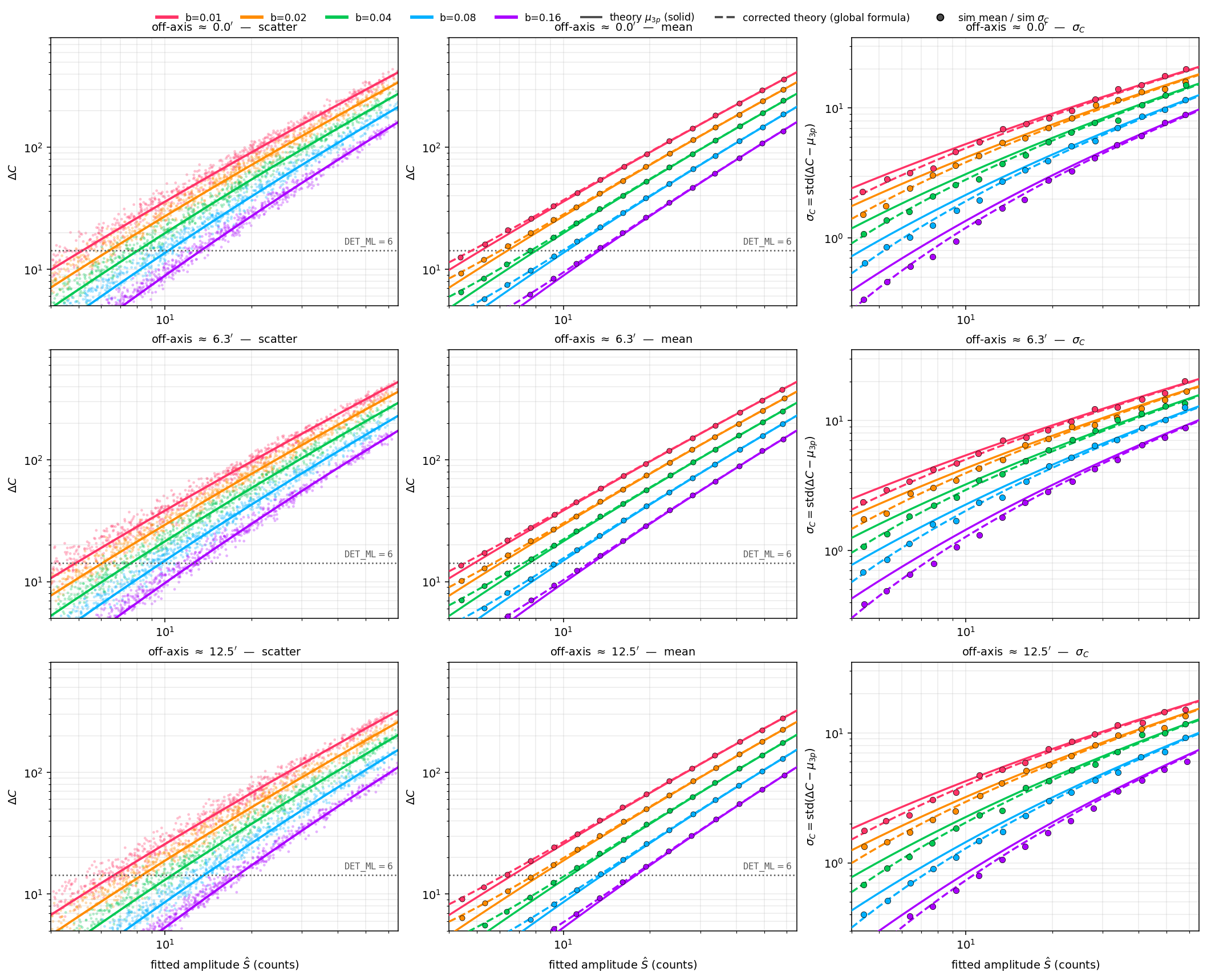
Figure [fig:deltac-scatter-variance] is the central validation diagnostic for the self-consistent reference-fitter theory. It shows, in one place, the three empirical facts on which the analytic part of the paper rests: the mean trend is captured by the observable-conditioned pixel-sum theory, the remaining low-signal bias is smooth, and the Fisher-projected variance gives the correct high-signal scale. The figure uses three representative off-axis rings (rows) and five backgrounds $b$ (colors). The left column shows individual $\Delta C_\mathrm{obs}$ values against $\widehat{S}$ with the theoretical conditional mean $\mu_{3p}(\widehat{S},b,\mathrm{psf},\mathrm{mask})$ overlaid; the $b$-stratified structure is regular and monotone. The middle column compares the binned simulation mean against $\mu_{3p}$: the asymptotic theory is accurate at high $\widehat{S}$ but carries a positive low-$\widehat{S}$ beyond-Fisher bias, which a global two-parameter correction removes. The right column shows the same decomposition for the residual scatter $\sigma_C = \sigma_{\Delta C - \mu_{3p}}$: the Fisher-projected $\sqrt{\sigma^2_{3p}}$ slightly overestimates the simulated scatter at low $\widehat{S}$, a deficit removed by the same type of global correction. The dashed lines are the single closed-form expressions of Equations ([eq:mean-corr])–([eq:sigma-corr]), applied identically across all three off-axis rings. The correction depends on $(\widehat{S}, b)$ only: an off-axis term is statistically negligible (Section 4.4), so the residual structure is governed by the fitted signal and background rather than by off-axis angle.

Reference-fitter validation results

Table [tab:ref-fitter-validation] summarizes the validation across fitted-signal ranges. At high signal ($\widehat{S}>20$), the standardized residual has $\langle Z \rangle = +0.07$ and $\sigma_Z = 0.98$, confirming closure of the theory. The stronger $\widehat{S}>50$ subset approaches zero mean and unit width even more closely, as expected for the Fisher/Gaussian approximation in the high-signal regime. At low fitted signal, a positive bias emerges: position optimization can absorb positive Poisson noise features, and the likelihood surface is less well approximated by a local quadratic expansion. This beyond-Fisher bias is not a grid artifact; it is a limitation of the Gaussian/Fisher approximation at low fitted signal.

Closed-form global corrections

The low-signal bias seen above admits a compact closed-form description. Binning the reference-fitter output in observable space by $\widehat{S}$ (using $\widehat{S}>4$ to constrain the low-signal end) across all 17 positions and 6 backgrounds, the mean residual and the residual-scatter ratio are each well described by a single $(\widehat{S},b)$ expression. These global expressions empirically support the interpretation that the beyond-Fisher residual is a smooth, low-dimensional function of $(\widehat{S},b)$, with no significant off-axis dependence (Section 4.4). This smoothness motivates the empirical grid-interpolation strategy deployed in Section 5: if the residual were erratic or high-dimensional, sparse-grid interpolation would fail. However, these specific closed-form global corrections remain strictly diagnostic and are not directly deployed in the final operational calibration. The standalone emldetect calibration absorbs all low-signal biases and implementation-specific effects entirely into the empirical $R_\mathrm{eml}$ grid.

The empirical status of these corrections is itself a constrained result, not merely a modeling convenience. Two direct verification tests, to be presented elsewhere, bracket simpler alternatives. First, a second-order expansion of $C_\mathrm{best}$ conditioned on the amplitude score, evaluated with no fitted coefficients, fails to reproduce the five coefficients in Equations ([eq:mean-corr])–([eq:sigma-corr]): its mean contribution is approximately a constant position-rank gain rather than the observed $\widehat{S}^{-0.40}$ decay, and its variance term does not yield the empirical $1/\widehat{S}$ scatter deficit. This places the low-signal residual beyond a local quadratic or Bartlett-type expansion, consistent with the position-argmax mechanism isolated in the reference-fitter decomposition. Second, a cross-PSF transferability test using Gaussian $\sigma=1.59$ pixel, broad Gaussian $\sigma=2.79$ pixel, and King $r_c=2.5$ pixel, $\alpha=1.5$ toy configurations with the same $\mathtt{ecut}=15$ mask shows that the correction coefficients are PSF-family specific: the Gaussian-toy mean law differs from the XMM-psfgen-template production law at high significance in the most precise low-$\widehat{S}$ bins, and neither $b A_\mathrm{psf}$ nor $b\,n_\mathrm{pix}$ collapses the mean coefficients across PSF families. Consequently, the low-signal correction must be calibrated per PSF-template family. Within the XMM psfgen-template family used here, the 17-position off-axis stability demonstrated below is precisely the validated operational domain.

Two further consequences of this PSF-family view, established in a pilot study on real psfgen templates spanning all three EPIC cameras and two energy bands prepared through a single template pipeline, are worth recording here. First, once the template preparation is unified, the per-instrument, per-band structure of the correction dissolves: the five coefficients reduce to a label-free form in which three are shared constants and two are smooth single-variable functions of scalar PSF features (the effective PSF area and the peak pixel fraction), with no instrument or band identifier remaining in the model. A full presentation of this reduced, label-free correction law is deferred to a follow-up paper. Second, and directly relevant to any application of the corrections in this paper: the absolute values of the correction coefficients depend on the PSF-template preparation convention (high-resolution sampling, rebinning, cropping, and normalization choices). Calibration and deployment must therefore use one and the same template pipeline; coefficients calibrated under one preparation convention must not be combined with templates prepared under another.

The conditional mean is corrected additively,

$$\mu_{3p}^\mathrm{corr}(\widehat{S},b) = \mu_{3p}(\widehat{S},b,\mathrm{psf},\mathrm{mask}) + \big(a_\mu + c_\mu\log_{10}b\big)\,\widehat{S}^{-p_\mu}, \label{eq:mean-corr}$$

with $a_\mu=0.59\pm0.12$, $c_\mu=-1.02\pm0.10$, $p_\mu=0.40\pm0.05$ (uncertainties from a position-level bootstrap; see below), and the residual scatter is corrected multiplicatively,

$$\sigma_C^\mathrm{corr}(\widehat{S},b) = \sqrt{\sigma^2_{3p}}\; \Big[\,1-\frac{a_\sigma + c_\sigma\log_{10}b}{\widehat{S}}\,\Big], \label{eq:sigma-corr}$$

with $a_\sigma=1.49\pm0.04$ and $c_\sigma=0.39\pm0.03$. The scatter correction has the form of a $1/\widehat{S}$ low-signal deficit that vanishes asymptotically, returning the Fisher-projected variance at high fitted signal. Equation ([eq:sigma-corr]) reduces the bin-level scatter of the empirical-to-theoretical $\sigma_C$ ratio from $0.074$ (uncorrected) to $0.049$, the residual being consistent with the Monte-Carlo uncertainty of the per-bin scatter estimate. A mild residual remains at the highest background ($b=0.16\,\mathrm{counts\,pixel^{-1}}$) and lowest fitted signal, where the empirical deficit is flatter in $\widehat{S}$ than the global form; this regime lies far below the $\mathrm{DET\_ML}=6$ detection threshold and does not affect the validated operational range.

Off-axis independence of the corrections

Both corrections in Equations ([eq:mean-corr])–([eq:sigma-corr]) depend on the fitted amplitude and background only. Adding a linear off-axis term $d\,\theta$ to the scatter model leaves the fit quality essentially unchanged ($d=-5\times10^{-3}$ per arcmin; the root-mean-square residual is unchanged to three decimal places), and the empirical $\sigma_C$ ratio is flat at $0.92$–$0.93$ across the full $0$–$14'$ off-axis range. The apparent “far-off-axis” variance offset is therefore not an off-axis effect: it is the low-$\widehat{S}$ deficit of Equation ([eq:sigma-corr]), seen more prominently in off-axis rings because those positions sample a larger fraction of low-$\widehat{S}$ fits. A single $(\widehat{S},b)$ correction suffices for all detector positions in the validated domain. This within-family stability, contrasted with the cross-family dependence described above, delineates the validity boundary of Equations ([eq:mean-corr])–([eq:sigma-corr]).

The coefficients are stable under the number of detector positions used in the fit. A position-level bootstrap (resampling the 17 positions with replacement, 400 realizations) recovers the central values quoted above and provides the uncertainties given for Equations ([eq:mean-corr])–([eq:sigma-corr]). Resampling random position subsets of fixed size $k$ leaves the central coefficients unchanged within scatter and shrinks their spread as $k^{-1/2}$, indicating that the positions sample the correction independently and without a systematic off-axis trend.

Limitations of the high-signal asymptotic closure and the role of empirical calibration

The sensitivity-map regime of interest is $\mathrm{DET\_ML}$ around 6–10, corresponding to $\Delta C \approx 14.3$–$22.8$. For the current PN band-4 setup at $b=0.04\,\mathrm{counts\,pixel^{-1}}$, this corresponds roughly to $\widehat{S}\sim 7.5$–$12.1$. This is strictly below the $\widehat{S} > 20$ high-signal validation range. We therefore state explicitly: the high-signal asymptotic closure of Section 4.2 does not directly validate the theory in the threshold band where it is operationally applied. In this low-signal regime, the threshold-band residual $R_\mathrm{eml}$ is treated via pure empirical interpolation.

Physically, $R_\mathrm{eml}$ originates from three sources: (i) the beyond-Fisher bias of the $\Delta C$ theory itself near the $S=0$ boundary, where the non-negativity constraint violates the interior-point assumption of Wilks’ theorem; (ii) implementation-specific artifacts of standalone emldetect, including its internal optimizer, PSF sampling, and numerical discretization details; and (iii) differences between the $\mathtt{ecut}=15$ fitting footprint used in the theory and the actual mask applied by the pipeline. Although $R_\mathrm{eml}$ is in principle a function of $S$, it varies slowly enough across the narrow threshold band ($\widehat{S} \sim 7$–$12$) that it is robustly approximated as a per-position scalar offset. Same-seed paired reference-fitter and standalone emldetect experiments show that the standalone $\Delta C$ tracks the reference fitter almost perfectly (correlation 0.996), with a small affine offset and an implementation jitter that grows with off-axis angle; this supports treating the transfer from the reference theory to the standalone pipeline as an empirical implementation layer rather than as a change to the observable-conditioning formalism.

A standard Monte Carlo fake-source injection approach (e.g., esensmap simulation mode) would capture all of these effects automatically: one simply injects sources at every sky position and background level, runs the full pipeline, and numerically tabulates the detection fraction. Such an approach delivers superior absolute accuracy because it makes no theoretical approximation. However, it is computationally prohibitive for continuous sky mapping across the full range of backgrounds, off-axis angles, and PSF geometries encountered in a survey-scale sensitivity map. Large modern surveys therefore often rely on extensive end-to-end simulations to characterize completeness, purity, and selection thresholds, as in the eROSITA eFEDS source-detection calibration .

The scientific value of the Section 3 theory is that it supplies the correct functional form of the observable-conditioned $\Delta C$ expectation as background, PSF geometry, and mask vary continuously across the detector. By anchoring the calculation to the deterministic theoretical mean $\mu_{3p}$, the operational calibration only needs to empirically determine the slowly-varying scalar residual $R_\mathrm{eml}$ on a sparse grid. This hybrid approach (analytic backbone plus empirical residual calibration) sacrifices the absolute accuracy of full Monte Carlo (yielding the 11–17% $S_\mathrm{lim}$ recovery errors reported in Section 5) but avoids the extreme computational cost of dense fake-source injection at every sky position. That operational calibration is the subject of Section 5.

Standalone emldetect Threshold Calibration

Section 4 established that the observable-conditioned $\Delta C$ theory closes when the data-generating model, fitting model, and theory are matched (the reference-fitter unit test for the analytic backbone). Standalone SAS emldetect introduces its own source fitting, optimizer, and PSF/model conventions; these implementation details produce a position-dependent residual relative to the reference theory. The difference between the reference-fitter closure and the standalone pipeline outcome is the target of the empirical calibration below. An empirical, position-dependent residual calibration absorbing this offset is constructed for the threshold regime $\mathrm{DET\_ML}=6$–10, applicable to standalone fake-source sensitivity-map work.

Empirical residual calibration

The raw theory predicts $$\mu_{3p}(\widehat{S},b,\mathrm{psf},\mathrm{mask}) = E[\Delta C | \widehat{S},b,\mathrm{psf},\mathrm{mask}]$$ If standalone emldetect exactly matched the same model, the threshold limit could be found from $$\mu_{3p}(S_{\mathrm{lim}},b,\mathrm{psf},\mathrm{mask}) = \Delta C_{\mathrm{th}}$$ In practice, this uncalibrated-theory baseline is only a borderline approximation in the threshold band. In the validation, it has maximum $S_\mathrm{lim}$ errors of 19.9% at $\mathrm{DET\_ML}=6$, 15.6% at $\mathrm{DET\_ML}=8$, and 13.3% at $\mathrm{DET\_ML}=10$. The error is position-dependent rather than a single scalar offset.

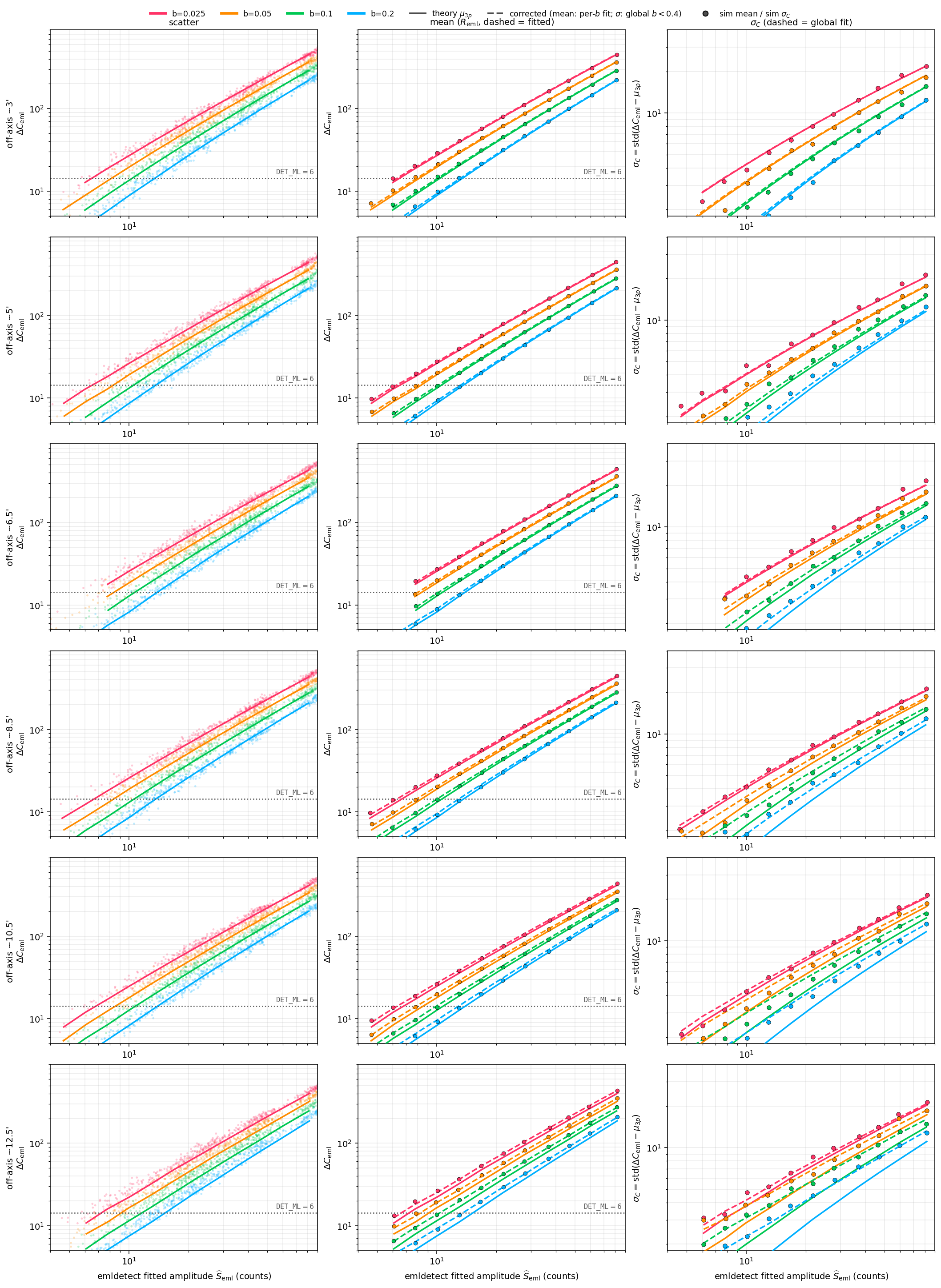
Figure [fig:emldetect-scatter-variance] is the central diagnostic for the operational standalone-emldetect chain. It is deliberately parallel to Figure [fig:deltac-scatter-variance]: the same observable-conditioned structure remains visible, but the standalone pipeline introduces a position-dependent residual relative to the reference-fitter theory. This is the visual reason that the final calibration is not the raw analytic equation, but the analytic equation plus an empirical $R_\mathrm{eml}$ calibration.

We therefore define the standalone emldetect residual

$$R_{\mathrm{eml}} = \Delta C_{\mathrm{eml}} - \mu_{3p}(\widehat{S}_{\mathrm{eml}},b,\mathrm{psf},\mathrm{mask}) \label{eq:reml}$$

Here $\Delta C_\mathrm{eml}$ is the standalone emldetect Cash improvement converted with the single-image $\nu=3$ convention, and $\widehat{S}_\mathrm{eml}$ is the fitted emldetect source amplitude. The calibrated threshold equation is

$$\mu_{3p}(S_{\mathrm{lim}},b,\mathrm{psf},\mathrm{mask}) = \Delta C_{\mathrm{th}} - \widehat{R}_{\mathrm{eml}} \label{eq:sensitivity-limit}$$

The sign follows directly from the residual definition. If $\widehat{R}_\mathrm{eml}>0$, standalone emldetect produces larger $\Delta C$ than the raw theory at the same fitted source strength, so the theoretical threshold needed for the sensitivity limit is lower. If $\widehat{R}_\mathrm{eml}<0$, the required source amplitude is higher.

The calibration uses paired fake-source simulations in which each realization is analyzed both by the reference fitter and by standalone SAS emldetect. The current calibration grid has 14 PN band-4 calibration positions after excluding the edge-affected case. The target threshold band is defined in $\Delta C$ space using the threshold conversions of Equation ([eq:detml-inverse]). Rows are selected by the reference-theory prediction: $$\mu_{3p,\mathrm{ref}} \in [\Delta C_{\mathrm{ML6}}, \Delta C_{\mathrm{ML10}}]$$ This is important: the threshold sample is not selected by observed $\mathrm{DET\_ML}_\mathrm{eml}$ or by observed $\Delta C_\mathrm{eml}$, because those quantities carry the stochastic fluctuation and implementation residual we are trying to calibrate. The selection is based on the predicted/reference $\Delta C$ in the observable-conditioned theory. The baseline calibration grid is built at $b = 0.04\,\mathrm{counts\,pixel^{-1}}$; background transfer to $b=0.02$ and $b=0.08\,\mathrm{counts\,pixel^{-1}}$ is included in the uncertainty budget below.

The residual $\widehat{R}_\mathrm{eml}$ is estimated at each detector position from the threshold-band simulation sample. Two interpolation schemes are compared: bilinear interpolation over the calibration grid in the adopted spatial coordinate (off-axis angle and a sector-coded calibration coordinate), and nearest-calibration-position assignment. The calibration coordinate is a sector-coded azimuthal label with four quadrant codes at 0, 90, 180, 270 degrees; it is a proof-of-concept operational coordinate, not a physical detector azimuth. A future production calibration should instead model $R_\mathrm{eml}$ as a function of physically motivated predictors, such as the local PSF second moment $A_2$, an effective PSF winginess parameter $W_\mathrm{eff}$, off-axis angle, and detector-edge distance, rather than categorical sector codes. The present sector coordinate suffices for the current 14-position grid because $R_\mathrm{eml}$ varies slowly enough across the narrow threshold band that the interpolation error is dominated by grid sparsity rather than by the coordinate choice.

Cross-validated accuracy

Validation uses leave-one-position-out cross-validation: each position is held out, the calibration is built from the remaining positions, and the predicted $S_\mathrm{lim}$ is compared to the held-out position’s internally calibrated reference limit. This held-out reference limit, $S_\mathrm{ref}$, is defined using the same reference fitter that is used throughout Section 4: for each simulated source strength, the median $\Delta C_\mathrm{fit}$ across repetitions is computed, a smooth interpolating spline is fitted to the median $\Delta C_\mathrm{fit}$ versus source-strength curve, and $S_\mathrm{ref}$ is defined as the exact root where the spline crosses $\Delta C_\mathrm{threshold}$. No information from the held-out position is permitted to leak into the $\widehat{R}_\mathrm{eml}$ interpolation model, ensuring a strict out-of-sample prediction test. We emphasize that this cross-validation tests the calibration’s ability to self-consistently interpolate the pipeline’s own threshold mapping across the calibration grid; it is not an absolute astrophysical validation against independent observational data or against injection-recovery detection fractions. Such absolute validation, for example comparing the predicted $S_\mathrm{lim}$ against an injection-recovery 50% completeness flux from dense fake-source injection at representative positions, is a necessary future step for production use. The reported error is

$$|S_{\mathrm{lim,pred}} - S_{\mathrm{ref}}| / S_{\mathrm{ref}}$$

Table [tab:unified-validation] consolidates the reference-fitter closure, the cross-validated $S_\mathrm{lim}$ accuracy, and the background transfer error into a single summary. At $\mathrm{DET\_ML}=6$, the preferred bilinear interpolation yields a median error of 4.1% and a maximum error of 11.0% for positions inside the calibration hull (10 of 14 held-out positions); the nearest-calibration-position assignment covers all 14 positions with a maximum error of 17.2%. Background transfer from $b=0.04\,\mathrm{counts\,pixel^{-1}}$ to the range $b=0.02$–$0.08\,\mathrm{counts\,pixel^{-1}}$ adds at most 5.7% error in $S_\mathrm{lim}$ at $\mathrm{DET\_ML}=6$. Both errors decrease at higher thresholds.

The uncalibrated theory has a maximum $S_\mathrm{lim}$ error of 19.9% at $\mathrm{DET\_ML}=6$ (7.2% median), making it only borderline as a standalone approximation at the most stringent threshold. A global scalar correction fails at $\mathrm{DET\_ML}=6$ (maximum error 21.6%), confirming that the residual is position-dependent. The bilinear interpolation within the calibration hull is the preferred method; outside the hull, the nearest-calibration-position assignment provides the validated all-position fallback.

Catalog Applications of the Conditional $\Delta C$ Distribution

The preceding sections calibrate the behavior of the likelihood-ratio statistic in $\Delta C$ space. The calibrated distribution has two catalog-level uses. The first is an interpretive use for traditional $\mathrm{DET\_ML}$-selected catalogs: the catalog may still be defined by an observed threshold, $\Delta C>\Delta C_\mathrm{th}$, but the forward distribution supplies the likelihood needed to infer the corresponding distribution of fitted source amplitudes. The second use is constructive: one can define catalog cuts directly in the fitted-amplitude coordinate by requiring a chosen percentile of the local $\Delta C$ distribution to reach the detection threshold. Both uses rely on the same forward kernel, but they use it in opposite directions (Table [tab:two-catalog-uses]).

Here $S$ denotes the source-amplitude coordinate used by the observable-conditioned theory, consistent with the fitted-amplitude convention used throughout this work. It is not an intrinsic injected flux.

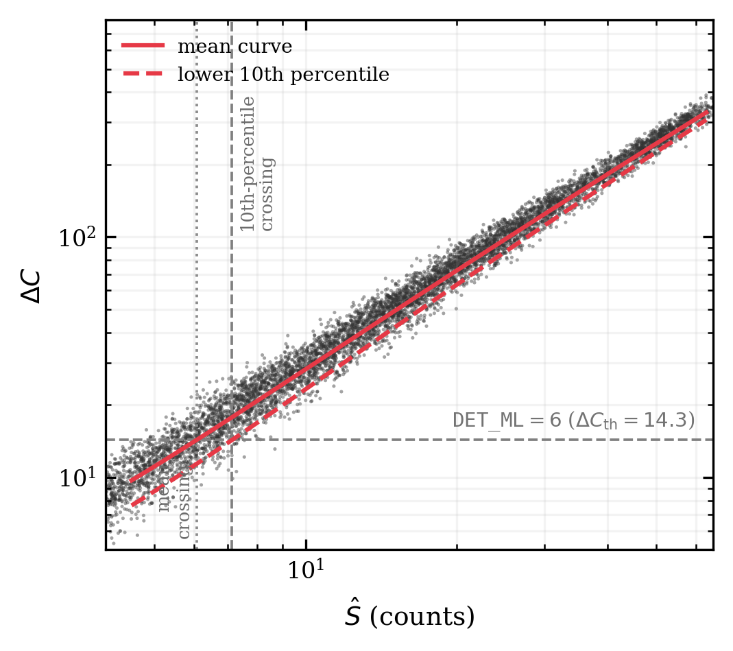
Figure 1 gives the visual version of the construction. A traditional $\mathrm{DET\_ML}$ threshold is a horizontal cut in $\Delta C$ space. Reading the conditional distribution backward from that cut gives the fitted-amplitude distribution of a traditional threshold-selected catalog, once a source-count prior is specified. Reading it forward gives percentile crossings: the usual sensitivity map is the mean crossing, while a lower-percentile crossing defines a more conservative fitted-amplitude threshold-crossing cut.

The forward kernel in $\Delta C$ space

For each detector position, the operational $\mathrm{DET\_ML}$ threshold is first converted to the corresponding single-image three-parameter $\Delta C$ threshold. For example, $\mathrm{DET\_ML}=6$ corresponds to $\Delta C_\mathrm{th}=14.3$ under the $\nu=3$ convention. The distributional calculation is then carried out in $\Delta C$ space; $\mathrm{DET\_ML}$ remains only the final operational threshold scale.

In the calibrated standalone-emldetect case, the mean of the forward kernel is

$$\Delta C_\mathrm{mean}(S,x,b) = \mu_{3p}(S,b,\mathrm{psf}_x,\mathrm{mask}_x) + \widehat{R}_\mathrm{eml}(x), \label{eq:mean-threshold-curve}$$

where $\widehat{R}_\mathrm{eml}$ is the empirical residual interpolated from the Section 5 calibration grid. With the Gaussian residual approximation, the local kernel is summarized as

$$p(\Delta C\mid S,x,b) \simeq \mathcal{N}\!\left[ \Delta C_\mathrm{mean}(S,x,b),\, \sigma_C^2(S,x,b) \right], \label{eq:deltac-forward-kernel}$$

and the corresponding $p$th percentile curve is

$$\Delta C_{p}(S,x,b) \simeq \Delta C_\mathrm{mean}(S,x,b) + z_p\,\sigma_C(S,x,b), \label{eq:deltac-percentile-curve}$$

where $z_p$ is the standard-normal quantile. The percentile construction requires, in addition to the calibrated mean residual, a calibrated threshold-band scatter model $\sigma_C$ in $\Delta C$ space. Thus $\Delta C_{50}\simeq \Delta C_\mathrm{mean}$, $\Delta C_{16}\simeq \Delta C_\mathrm{mean}-\sigma_C$, $\Delta C_{10}\simeq \Delta C_\mathrm{mean}-1.282\,\sigma_C$, and $\Delta C_{2.3}\simeq \Delta C_\mathrm{mean}-2\,\sigma_C$.

In the present proof-of-concept application, we use the empirically corrected scatter model from Section 4 as the distributional backbone. The Fisher-projected variance supplies the analytic scale, but production use of the full kernel or of lower-percentile maps requires direct validation against standalone-emldetect passing fractions, because the high-signal reference-fitter closure does not by itself validate the $\mathrm{DET\_ML}=6$–10 threshold band.

Application I: interpreting traditional $\mathrm{DET\_ML}$-selected catalogs

The first application keeps the traditional catalog definition. A source is selected by an observed detection statistic, for example $\mathrm{DET\_ML}>T$, equivalently $\Delta C>\Delta C_\mathrm{th}$. The new ingredient is that the catalog threshold can now be interpreted through the forward kernel in Equation ([eq:deltac-forward-kernel]).

For a source with a measured value $\Delta C_\mathrm{obs}$, the fitted-amplitude posterior in catalog space is

$$p(S\mid \Delta C_\mathrm{obs},x,b) \propto p(\Delta C_\mathrm{obs}\mid S,x,b)\,\pi(S), \label{eq:posterior-single-source}$$

where $\pi(S)$ is a source-count prior expressed in the fitted-amplitude coordinate. For a threshold-selected ensemble, the analogous expression is

$$p(S\mid \Delta C>\Delta C_\mathrm{th},x,b) \propto P(\Delta C>\Delta C_\mathrm{th}\mid S,x,b)\,\pi(S), \label{eq:posterior-threshold-selected}$$

with

$$P(\Delta C>\Delta C_\mathrm{th}\mid S,x,b) = \int_{\Delta C_\mathrm{th}}^\infty p(\Delta C\mid S,x,b)\,d\Delta C . \label{eq:threshold-passing-probability}$$

Under the Gaussian residual approximation, this passing probability is a normal survival function evaluated in $\Delta C$ space. This route does not replace the traditional $\mathrm{DET\_ML}$ threshold. Instead, it adds the missing likelihood layer needed to interpret the fitted-amplitude distribution of a $\mathrm{DET\_ML}$-selected catalog. This is also the point at which Eddington bias enters: the noisy threshold statistic must be combined with a source-count prior, especially when the underlying $dN/dS$ is steep . A specified $\mathrm{DET\_ML}$ value or threshold therefore does not by itself define a flux distribution; it defines a likelihood factor in $\Delta C$ space. To obtain $p(S\mid \Delta C_\mathrm{obs})$ or $p(S\mid \Delta C>\Delta C_\mathrm{th})$, one must combine that likelihood with a source-count prior, for example a power-law $dN/dS$ slope or index expressed in the fitted-amplitude coordinate. Because this is an inverse problem, it necessarily depends on the population prior. If the desired prior is an intrinsic $dN/dS_\mathrm{true}$ rather than a prior in fitted catalog amplitude, an additional measurement model connecting $S_\mathrm{true}$ to the fitted amplitude $S$ is required.

The corresponding sky coverage is therefore probabilistic rather than a step-function area from a single limiting amplitude. At a given pixel $j$, detecting a source with fitted amplitude $S$ has the catalog-space density

$$q_j(S) \propto P(\Delta C>\Delta C_\mathrm{th}\mid S,x_j,b_j)\,\pi(S), \label{eq:pixel-detected-amplitude-density}$$

up to normalization over the fitted-amplitude coordinate. Thus the traditional threshold catalog assigns a probability to detected amplitudes at each pixel, rather than a single deterministic limiting amplitude. The corresponding effective area at fitted amplitude $S$ is

$$\Omega_\mathrm{th}(S) = \sum_j \Omega_j\, P(\Delta C>\Delta C_\mathrm{th}\mid S,x_j,b_j), \label{eq:traditional-probabilistic-sky-coverage}$$

where $j$ indexes sky or detector pixels. If the goal is the expected number of detected fitted amplitudes in an interval $A$, the same probability-weighted area is combined with the source-count prior,

$$N_\mathrm{det}(A) \propto \int_A \Omega_\mathrm{th}(S)\,\pi(S)\,dS . \label{eq:traditional-detected-amplitude-distribution}$$

This is the sense in which the sky coverage for Application I follows the probability distribution of detected fitted amplitudes, whereas the percentile-cut construction below starts from a chosen fitted-amplitude threshold-crossing probability.

Application II: fitted-amplitude percentile cuts

The second application uses the same kernel in the forward direction. Instead of starting from a noisy $\mathrm{DET\_ML}$-selected sample and asking what fitted amplitudes it contains, one asks what fitted amplitude is required for a specified fraction of realizations to exceed the detection threshold. This map-construction step fixes $S$ and evaluates $P(\Delta C>\Delta C_\mathrm{th}\mid S,x,b)$, so no $dN/dS$ slope or source-count index is required.

The usual sensitivity-map calculation is recovered as the mean-curve crossing

$$\Delta C_\mathrm{mean}(S,x,b)=\Delta C_\mathrm{th}. \label{eq:mean-curve-crossing}$$

Under a symmetric Gaussian residual approximation, this is also the 50th-percentile threshold-crossing point. We avoid calling it an empirical 50% completeness flux, because injection-recovery completeness is usually defined as $P(\mathrm{detected}\mid S_\mathrm{true})$ in the injected-flux coordinate.

More conservative fitted-amplitude cuts are obtained by solving the threshold equation with lower percentile curves,

$$\Delta C_p(S,x,b)=\Delta C_\mathrm{th}, \label{eq:percentile-threshold-crossing}$$

with $p<50$. The direction is important. Requiring 90% of realizations at a given fitted amplitude to exceed the threshold uses the lower 10th percentile, not the upper 90th percentile:

$$\Delta C_{10}(S,x,b)=\Delta C_\mathrm{th}.$$

Similarly, using the $\mu-2\sigma$ lower envelope corresponds to an approximately 97.7% threshold-crossing criterion under the Gaussian approximation. Table [tab:threshold-crossing-terms] summarizes the terminology used here.

Sky coverage for fitted-amplitude threshold-crossing cuts

Applying the same crossing rule to every detector pixel produces a family of fitted-amplitude sensitivity maps: a mean-threshold map, an 84% threshold-crossing map from the lower 16th percentile, a 90% threshold-crossing map from the lower 10th percentile, and so on. Each map can be converted into a threshold-crossing sky-coverage curve by counting the sky area over which the local limiting amplitude is below a trial fitted amplitude,

$$\Omega_p(S) = \sum_j \Omega_j\, I\!\left[S_\mathrm{lim}^{(p)}(j) \le S\right],$$

where $j$ indexes sky or detector pixels and $p$ denotes the percentile curve used in Equation ([eq:percentile-threshold-crossing]). This threshold-crossing sky-coverage calculation is an instrumental, catalog-space quantity in the same fitted-amplitude coordinate used by the observable-conditioned theory: it depends on the local background, PSF, mask, threshold, and residual calibration, but it does not require an assumed $dN/dS$ slope. A source-count model is needed only in the subsequent population inference.

Relation between the two uses and Eddington bias

Both applications come from the same conditional distribution $p(\Delta C\mid S,x,b)$, but they answer different questions. Application I is backward: it starts from an observed $\mathrm{DET\_ML}$ value or a $\mathrm{DET\_ML}$-selected catalog and infers the fitted-amplitude distribution. This is the natural setting for Eddington-bias modeling, because the asymmetry near a detection threshold is produced by combining the noisy threshold statistic with a steep source-count prior.

Application II is forward: it starts from a fitted amplitude and asks for the probability of crossing the $\mathrm{DET\_ML}$ threshold. This does not remove population-level Eddington bias from a luminosity-function inference, but it allows one to construct an instrumental catalog-space subsample with an explicitly stated threshold-crossing probability. In this sense, the percentile sensitivity map is a catalog-construction tool, whereas the threshold-selected posterior is a catalog-interpretation tool.

Validation requirements and limitations

The cross-validation in Section 5 validates the mean/median-threshold fitted-amplitude mapping: at $\mathrm{DET\_ML}=6$, the preferred bilinear interpolation reaches a maximum error of 11.0% inside the calibration hull, while the nearest-calibration-position fallback reaches 17.2% across all held-out positions. The two applications above require additional validation beyond this mean-crossing test. For Application I, the likelihood kernel should be tested against the observed distribution of standalone-emldetect $\Delta C$ values in held-out simulations. For Application II, the scatter and tail model should be validated by comparing the predicted threshold-crossing probability against the empirical detection fraction, binned for example near predicted probabilities of 0.5, 0.7, and 0.9. Agreement of the empirical passing fraction with the predicted probability is the necessary validation for using lower-percentile maps as catalog threshold-crossing sensitivity cuts.

Thus the application presented here is a fast, distributional, catalog-oriented framework for threshold interpretation and fitted-amplitude threshold-crossing sensitivity. Full injection-recovery simulations remain the absolute validation standard for production selection functions in complex survey fields.

The calibration grid, cross-validation tables, figure-generation scripts, configuration files, and minimal scripts reproducing key validation results will be made available upon publication via a persistent Zenodo archive.

Scope and Limitations

The presented framework focuses on methodological advances: the conditional-mean formula, the Fisher-projected variance, and the observable-conditioning principle transfer algebraically to any Poisson PSF-fitting source-detection pipeline that employs a standard three-parameter fit; however, quantitative use requires pipeline-specific recalibration. Furthermore, the quantitative calibration (specifically the position-dependent residual grid, the leave-one-out cross-validation error budgets, and the threshold-crossing fitted-amplitude mapping) has been validated exclusively via single-image fake-source simulations in the XMM-Newton PN band-4 setting. Applying this approach to different instruments, energy bands, or detection pipelines will necessitate a re-derivation of the pipeline-specific likelihood transformation and a complete re-calibration of the implementation residuals using matched fake-source grids.

While the self-consistent reference-fitter confirms the theoretical model structure in the high-signal regime ($\widehat{S} > 20$), these results cannot be blindly extrapolated to the threshold band ($\mathrm{DET\_ML}\approx 6$–10). At lower fitted signals ($\widehat{S} \lesssim 12$), the reference fitter exhibits a positive beyond-Fisher bias. The standalone calibration absorbs this bias along with other algorithmic effects into the empirical $R_\mathrm{eml}$ residual, yielding an operational prediction for the local $\Delta C$ and $\mathrm{DET\_ML}$ distribution.

Furthermore, we emphasize that our empirical calibration is not a comprehensive correction for the official XMM-Newton serendipitous source catalogs (e.g., 4XMM). The catalog environments involve complexities such as complex background map variations, multi-observation stacking, vignetting weighting, and source-confusion effects that are not fully captured by our single-image standalone simulations. Other current X-ray catalog pipelines handle related complications with substantially different machinery, for example the eROSITA eSASS/eFEDS simulation-calibrated detection chain and the Chandra Source Catalog Release 2 series with co-added observations, local PSF modeling, and Bayesian aperture photometry . These examples reinforce that the residual calibration developed here is pipeline-specific.

Regarding spatial interpolation, bilinear interpolation within the calibration hull provides the smallest errors, while nearest-calibration-position assignment supplies the validated all-position fallback. The adopted sector coordinate is a calibration coordinate rather than a physical detector azimuth. The calibration maintains a weak background dependence; transferring the $b=0.04\,\mathrm{counts\,pixel^{-1}}$ calibration to a background level of $0.08\,\mathrm{counts\,pixel^{-1}}$ introduced up to a 5.7% error in the inferred sensitivity limit, indicating that extrapolation to substantially different backgrounds without re-calibration should be avoided.

If no $R_\mathrm{eml}$ calibration grid is available, the uncalibrated theory may be used as an approximate estimate, with a maximum $S_\mathrm{lim}$ error of 19.9% at $\mathrm{DET\_ML}=6$. This is a fallback, not the recommended calibrated method. If the target setup differs from the validated domain, the calibration should be treated as unvalidated. Examples include: MOS instruments; merged images or multi-image fits; fixed-position fits with a different number of degrees of freedom; backgrounds outside the tested $b=0.02$–$0.08\,\mathrm{counts\,pixel^{-1}}$ range; PSF or mask conventions not matching the calibration grid; or official 4XMM catalog products.

Finally, Section 6 separates two uses of the same forward kernel. The backward interpretation of traditional $\mathrm{DET\_ML}$-selected catalogs is a population-inference problem and requires a source-count prior. The forward fitted-amplitude percentile maps do not require such a prior at the map-construction stage, but source-count and Eddington-bias corrections still require an assumed or fitted source-flux distribution and, where needed, a measurement model connecting intrinsic and fitted flux.

Conclusions

The conditional mean of the Cash-statistic improvement at a fitted source,

$$\mu_{3p}(\widehat{S}, b, \mathrm{psf}, \mathrm{mask}) = E[\Delta C | \widehat{S}, b, \mathrm{psf}, \mathrm{mask}],$$

is derived in closed form for the standard three-parameter (one amplitude, two position) single-source PSF fit under the SAS single-image convention ($\nu=3$, $\mathrm{shape}=1.5$; $\mathrm{DET\_ML}=-\ln Q(1.5,\,\Delta C/2)$, so that $\mathrm{DET\_ML}=6,\,8,\,10$ correspond to $\Delta C = 14.3,\ 18.6,\ 22.8$). Treating $\Delta C$ as a sampling distribution rather than as a single deterministic value is what distinguishes this framework from the prior analytical-mean sensitivity-map literature.

Self-consistent psfgen-template reference-fitter simulations spanning 17 PN band-4 detector positions ($\sim 8\times 10^5$ fits) close the predicted mean to within 0.07$\sigma$ and the Fisher-projected variance to within ${\sim}5$% in the high-signal regime ($\widehat{S} > 20$). The threshold band $\mathrm{DET\_ML}=6$–10 lies at lower fitted signal (roughly $\widehat{S}\sim 7.5$–$12.1$ at $b=0.04\,\mathrm{counts\,pixel^{-1}}$), where an asymptotic low-signal bias and an implementation-dependent residual of standalone SAS emldetect require an empirical, position-dependent residual calibration $R_\mathrm{eml}$. The validated mean/50th-percentile crossing equation

$$\Delta C_\mathrm{mean}(S,b,\mathrm{psf},\mathrm{mask}) = \Delta C_\mathrm{th}$$

reproduces the held-out reference limiting amplitude to within 11% (preferred bilinear interpolation, 10/14 in-hull held-out positions) and 17% (nearest-calibration-position fallback, all 14 positions) at $\mathrm{DET\_ML}=6$ on the PN band-4 calibration grid, with weak background dependence over $b=0.02$–$0.08\,\mathrm{counts\,pixel^{-1}}$ (maximum tested transfer error 5.7%). The adopted sector coordinate is a calibration coordinate, not a physical detector azimuth.

For catalog work, the calibrated kernel can be used in two directions. Backward, it supplies likelihood factors such as $p(\Delta C_\mathrm{obs}\mid S,x,b)$ or $P(\Delta C>\Delta C_\mathrm{th}\mid S,x,b)$ for interpreting traditional $\mathrm{DET\_ML}$-selected catalogs with a source-count prior. Forward, it gives the local fitted-amplitude threshold-crossing probability $P(\mathrm{DET\_ML}>T\mid S,x,b)$. A 90% threshold-crossing fitted-amplitude limit, for example, is the source amplitude for which the 10th percentile of the predicted $\Delta C$ distribution equals the detection threshold. Sky area as a function of fitted amplitude then follows by counting the detector pixels satisfying the chosen threshold-crossing condition.

The methodological core is independent of XMM-Newton: the observable-conditioned $\Delta C$ theory for the three-parameter Poisson PSF source fit, and the threshold calibration in $\Delta C$ residual space rather than in pipeline-reported detection-statistic space. Extension to other Poisson PSF-fitting source-detection pipelines is a natural follow-up; the XMM-Newton emldetect results above are the first concrete validation and calibrated application within the framework.

Data and Code Availability

The calibration grid, cross-validation tables, figure-generation scripts, SAS configuration files, and minimal scripts reproducing key validation results (including the exact commands, random seeds, psfgen parameters, and emldetect invocation flags) are deposited in a Zenodo archive. A private review link is available; the final DOI will be inserted upon acceptance.

The calibration grid is provided as a machine-readable table. The code is released under an open-source license.

Diagnostic role of injected source strength

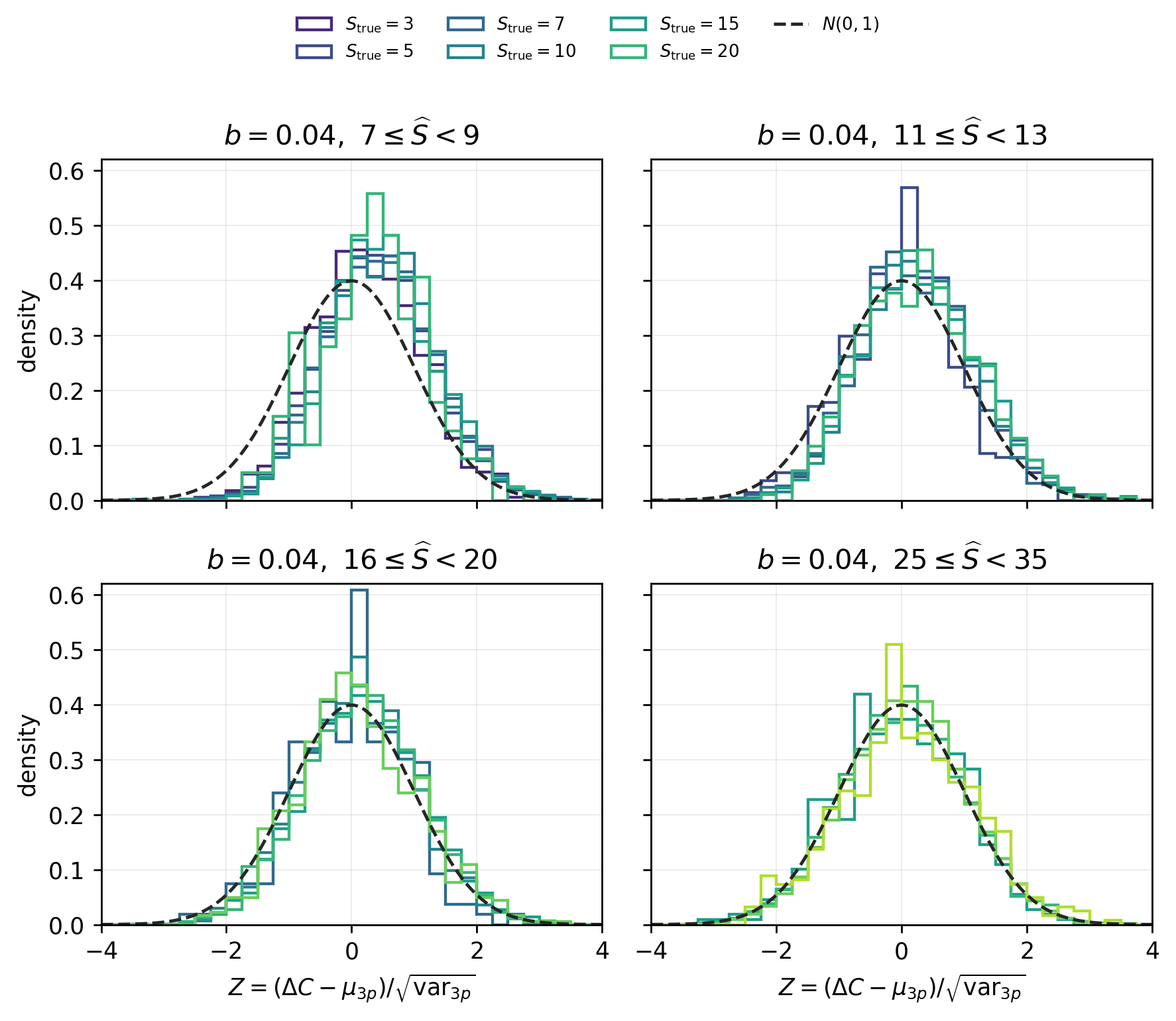
Figure 2 is a diagnostic check on the conditioning variable. The simulations know the injected source strength $S_\mathrm{true}$, but the theory and the operational calibration condition on the fitted amplitude $\widehat{S}$. At fixed detected $\widehat{S}$, the standardized residual distributions from different $S_\mathrm{true}$ subsets overlap closely. The residual offset in the lowest $\widehat{S}$ bin is the same low-signal beyond-Fisher bias discussed in Section 4.2, not evidence for conditioning on $S_\mathrm{true}$.

Acknowledgments

We acknowledge support from the National Natural Science Foundation of China. This research has made use of data obtained from the XMM-Newton satellite, an ESA science mission with instruments and contributions directly funded by ESA Member States and NASA.

参考文献

(参考文献列表见源文件)