Introduction

泊松源探测以 Delta C 和检测似然选择目录源 / Poisson source detection uses Delta C and detection likelihood to select catalog sources

Source detection in Poisson-count photon imaging is commonly carried out by fitting a parametric source model on top of a known background and summarizing the result by a likelihood-ratio statistic. Under the standard Cash-statistic formulation (Cash 1979), the natural statistical object is the Cash improvement $\Delta C = C_\mathrm{null} - C_\mathrm{best}$, with $C$ proportional to twice the negative Poisson log-likelihood. Detection pipelines typically report a monotone transform of $\Delta C$ as a “detection likelihood”; in the XMM-Newton Science Analysis System, for example, emldetect (Cruddace et al. 1988; Watson et al. 2009) fits a three-parameter source model (one free amplitude and two free position coordinates) to Poisson-count images and reports $\mathrm{DET\_ML}$, an incomplete-gamma transform of the underlying $\Delta C$. The reported detection-likelihood statistic is operationally important: it is used to decide which sources enter a catalog, to define detection thresholds, and to construct sensitivity maps.

X射线巡天已广泛发展探测统计并采用 emldetect / X ray surveys developed extensive detection statistics and use emldetect

Sensitivity maps and source counting methodologies have been extensively developed and applied in major X-ray surveys (Cappelluti et al. 2009; Georgakakis et al. 2008; Laird et al. 2009; Luo et al. 2017, e.g.,; Mateos et al. 2008; Puccetti et al. 2009; Wang et al. 2016; Xue et al. 2011). The statistical treatment of Poisson source detection, limits, and likelihood ratio methods also has a long history in high-energy astrophysics (Broos et al. 2010, e.g.,; Gehrels 1986; Kashyap et al. 2010; Kraft et al. 1991; Protassov et al. 2002; Starck et al. 2002). The emldetect tool has been the standard for the XMM-Newton serendipitous survey catalogs (Carrera et al. 2007; Rosen et al. 2016; Traulsen et al. 2019; Watson et al. 2009; Webb et al. 2020).

DET ML 仅作阈值尺度而非已校准零假设概率 / DET ML is only a threshold scale not a calibrated null probability

We use $\mathrm{DET\_ML}$ strictly as the operational monotone threshold scale defined by SAS, not as a calibrated frequentist false-alarm probability. The usual $\chi^2_3$ null reference assumes interior regularity, although source amplitude lies on a boundary and position is unidentifiable under the null (Chernoff 1954; Protassov et al. 2002; Self & Liang 1987). Monte Carlo experiments by Stewart (2009) found that the corresponding Cash-statistic reference can nevertheless be a good practical approximation under representative X-ray source-search conditions after negative-amplitude solutions are excluded. The low-count Cash statistic can also depart from its high-count limit (Bonamente 2020). We do not attempt to resolve that null-calibration debate. The conversion between $\mathrm{DET\_ML}$ and $\Delta C$ is used only to translate a chosen pipeline threshold into the statistic whose conditional distribution is modeled below.

低信号阈值处的波动和 Eddington 偏差影响极限流量 / Low signal fluctuations and Eddington bias alter limiting flux near threshold

The practical threshold regime is low signal. For many XMM-Newton applications the relevant sensitivity-map range is $\mathrm{DET\_ML}$ of order 6–10. This is the regime where source counts are steep, Poisson fluctuations matter, and a small shift in the detection threshold can change the inferred limiting flux. It is therefore also the regime where Eddington bias becomes important: random upward fluctuations are preferentially selected near the detection boundary, and the selected sample no longer represents the untruncated parent distribution (Eddington 1913; Wang 2004).

现有均值理论缺少三参数条件宽度及阈值传播 / Existing mean theory lacks three parameter conditional width and threshold propagation

The analytical mean is not the missing result. Stewart (2009) derived an amplitude-only Cash-statistic expectation and proposed its use in sensitivity calculations, extending earlier matched-filter sensitivity work (Stewart 2006). SAS esensmap likewise uses an emldetect-style analytical Cash model, following the 3XMM and 4XMM pipelines (Rosen et al. 2016; Traulsen et al. 2019); the New-ANGELS XMM survey evaluated a related expectation at the fitted rather than injected flux (Huang et al. 2025, appendix). Moments of the Cash statistic have also been derived for spectral goodness-of-fit problems (Kaastra 2017), a different estimand from the source-versus-background improvement studied here.

本文以位置尺度理论加低计数经验修正构建模型 / We combine location scale theory with low count empirical corrections

The unresolved quantity in these sensitivity calculations is the conditional width of the source-detection improvement. Among the X-ray sensitivity-map methods reviewed here, we find no previous explicit pixel-sum variance for $\Delta C$ after the amplitude and two position directions have been fitted, nor a threshold calculation that propagates that width in fitted-observable space. We therefore separate the problem into an analytical location and scale and an empirical low-count correction. The Asimov/Kullback–Leibler term supplies the location, while a Fisher/Wald projection supplies the leading variance (Cowan et al. 2011; Wilks 1938). This is the pixelized Poisson-imaging counterpart of related Fisher analyses of joint photometry and astrometry (Mendez et al. 2014).

模型架构通用但经验系数依赖具体拟合配置 / The architecture is general but empirical coefficients depend on the fitting configuration

The resulting model has a common architecture but not a universal set of empirical coefficients: $$\Delta C\mid\widehat S,b,\mathcal{P},\mathcal{M},k \simeq \mathcal{N}\!\left[ \mu_{3p}+\sqrt{V_{3p}}F_k(\mu_{3p}), V_{3p}G_k^2(\mu_{3p}) \right]. \label{eq:master-kernel}$$ Here $\mathcal{P}$ and $\mathcal{M}$ denote the pixelized PSF and fitting mask, and $k$ denotes the effective fitter/search configuration. The functions $F_k$ and $G_k$ describe the low-count location and width corrections. They must be estimated independently: a correct mean is needed to remove within-bin gradients before measuring the width, but it does not determine that width. The nonlinear incomplete-gamma transform from $\Delta C$ to $\mathrm{DET\_ML}$ is applied only after this distribution is constructed.

后续章节依次说明条件规则 理论 验证 标定和应用 / The following sections present conditioning theory validation calibration and applications in order

Section 2 fixes the observable-conditioning and selection rules. Section 3 derives the analytical location and Fisher-projected variance. Section 4 validates the reference-fitter kernel, including separate low-count corrections to the mean and width. Section 5 retains standalone emldetect as a pipeline-specific calibration case study and quantifies the cross-configuration transfer boundary. Section 6 develops fitted-amplitude threshold-crossing and catalog-inference consequences. Sections 7 and 8 state the evidence tiers and conclusions.

Observable-Conditioned Residuals

核心对象是在拟合观测空间中的条件 Delta C 分布 / The central object is the conditional Delta C distribution in fitted observable space

The central statistical object is the conditional distribution of $\Delta C$ in fitted-observable space,

$$p(\Delta C\mid \widehat{S},b,\mathcal{P},\mathcal{M},k).$$

where $\widehat{S}$ is the fitted source amplitude, $b$ is the local background in counts per pixel, $\mathcal{P}$ is the pixelized PSF template used by the fitting model, $\mathcal{M}$ is its image support, and $k$ records the remaining search and optimizer convention. Section 3 derives the leading location and variance. Section 4 measures the low-count corrections in a matched reference fitter, Section 5 examines a standalone pipeline calibration, and Section 6 states the uses and additional assumptions required for a selection function.

Conditioning on fitted amplitude

真实流量仅用于生成诊断 条件核按拟合振幅定义 / True flux serves only diagnostics and fitted amplitude defines the conditional kernel

In simulations, $S_\mathrm{true}$ is a generation label and is the appropriate conditioning variable for a separate generative selection model $p(\widehat S,\Delta C\mid S_\mathrm{true})$. It is not observed for catalog sources and is not the conditioning variable of the fitted-observable kernel developed here. We therefore use $S_\mathrm{true}$ only for generative diagnostics and condition all $\Delta C$ moment estimates on $\widehat S$; true-flux completeness is treated separately in Section 6. A result conditioned on $S_\mathrm{true}$ tests behavior at a known injected flux, whereas a result conditioned on $\widehat S$ tests the kernel after a source has been fit. Only the latter is the estimand of the observable-conditioned kernel and fitted-amplitude crossing maps studied here.

Residual decomposition

每个试验以观测拟合量计算理论位置并定义残差 / Each trial evaluates the theoretical location at fitted observables and defines a residual

For each source or fake-source trial the theory prediction is evaluated at the observed fitted quantities,

$$\mu_{3p,i} \equiv \mu_\mathrm{Asimov}(\widehat S_i,b_i,\mathrm{psf}_i,\mathrm{mask}_i) \simeq E[\Delta C\mid\widehat S_i,b_i,\mathrm{psf}_i,\mathrm{mask}_i]$$

and the residual is

$$R_{i} = \Delta C_{i} - \mu_{3p,i}.$$

样本方差包含残差位置和协方差三项 / Sample variance contains residual location and covariance contributions

For a sample or bin,

$$\begin{aligned} \langle \Delta C \rangle &= \langle R \rangle + \langle \mu_{3p} \rangle, \\ \mathrm{Var}(\Delta C) &= \mathrm{Var}(R) + \mathrm{Var}(\mu_{3p}) + 2\,\mathrm{Cov}(R, \mu_{3p}) \end{aligned}$$

宽度须在局部均值去除后估计且不得按检测量截断 / Width must be estimated after local mean removal without detection based truncation

Only when $\mu_{3p}$ is approximately constant across the bin does the observed $\Delta C$ variance reduce to $\mathrm{Var}(R)$; mixed-$\widehat{S}$ or mixed-position samples otherwise introduce apparent variance effects that are not properties of the conditional theory. We therefore estimate a local conditional mean in the same cells used for the width and compute the standard deviation only after subtracting that local trend. The mean is essential to this step, but the remaining width is an independent statistical target. Binning by $S_\mathrm{true}$ instead mixes fitted amplitudes and can inflate the apparent position dependence. Binning after a cut on observed $\mathrm{DET\_ML}$, $\Delta C$, or the residual is worse: it truncates the distribution whose moments are being estimated. Neither operation is used in the validation below.

Threshold selection in $\Delta C$ space

阈值先在 Delta C 空间定义以避免 DET ML 截断偏差 / Thresholds are defined in Delta C space to avoid DET ML truncation bias

$\mathrm{DET\_ML}$ is a nonlinear monotone tail-probability transform of $\Delta C$,

$$\mathrm{DET\_ML}= -\ln Q(\nu/2, \Delta C/2),$$

with $\nu=3$ and $\mathrm{shape}=1.5$ for the single-source three-parameter fit. The corresponding inverse is $$\Delta C_{\mathrm{th}} = 2\,Q_x^{-1}(1.5, \exp(-\mathrm{DET\_ML})), \label{eq:detml-inverse}$$ where $Q$ is the regularized upper incomplete gamma function and $Q_x^{-1}$ denotes inversion with respect to its second argument. Thus $\mathrm{DET\_ML}=6,\,8,\,10$ correspond to $\Delta C_{\mathrm{th}}=14.3,\,18.6,\,22.8$, respectively. A Gaussian residual in $\Delta C$ is therefore not Gaussian in $\mathrm{DET\_ML}$, and selecting on observed $\mathrm{DET\_ML}$ is a selection on the same noisy quantity whose distribution is being measured: it truncates the residual distribution and biases its mean upward near the threshold. Threshold ranges are accordingly translated into $\Delta C$ using the three-parameter convention and applied as theoretical or predicted $\Delta C$ conditions (such as $\mu_{3p,\rm ref}\in[\Delta C_\mathrm{ML6},\Delta C_\mathrm{ML10}]$) or as $\widehat{S}$ bins whose typical predicted $\Delta C$ lies in that interval. This keeps the conditioning independent of the observed stochastic fluctuation in $\Delta C_\mathrm{eml}$.

Analytic Conditional Location and Fisher-Projected Variance

本节推导三参数条件位置与投影方差 / This section derives the three parameter conditional location and projected variance

The Kullback–Leibler/Asimov construction for the location and the Fisher/Wald construction for local fluctuations are standard likelihood tools (Cowan et al. 2011; Wilks 1938). Their evaluation for a pixelized Poisson source fit yields the specific result needed here: an explicit variance after the amplitude and both position score directions have been removed. We derive the location and this projected variance for one free amplitude and two free coordinates. The variance, rather than the analytical mean alone, is the main theoretical contribution.

Pixelized Poisson model

像素化泊松计数构成拟合区域的观测模型 / Independent pixel Poisson counts define the fitting region observation model

Consider a fitting region containing pixels indexed by $i$. The observed counts are independent Poisson random variables,

$$Y_{i} \sim \mathrm{Poisson}(\mu_i)$$

单源拟合模型结合背景振幅和二维 PSF 位置 / The fitted single source model combines background amplitude and two dimensional PSF position

For a single source on a locally known background, the fitted source model is

$$\begin{aligned} \mu_i(\theta) &= b_{i} + S\, p_{i}(x, y), \\ \theta &= (S, x, y) \end{aligned}$$

Here $b_i$ is the background expectation in pixel $i$, $S$ is the source amplitude in the same units used by the image model, and $p_i(x,y)$ is the pixelized PSF template shifted to position $(x,y)$. The PSF is normalized over the full template grid, $\sum_i p_i=1$; the mask $M_i$ then selects the fitting footprint. Thus $S$ denotes the total source amplitude in the template convention, not the counts enclosed by the fitting mask. In the current PN band-4 validation runs, $b_i$ is usually a constant $b$ inside the fitting region, but the notation allows the background to vary by pixel.

二元掩膜定义拟合像素并连接加权掩膜扩展 / A binary mask selects fitted pixels and connects to the weighted mask extension

A binary fitting mask $M_i$ selects the pixels included in the fit; the primary results in this paper use binary masks. A weighted-mask extension exists for fractional weights, but when the weights are exactly 0 or 1 the weighted formula reduces to the binary-mask convention used here.

Cash statistic and $\Delta C$ sign convention

Cash 统计量定义为掩膜像素的泊松似然量 / The Cash statistic is defined from the masked pixel Poisson likelihood

Ignoring constants independent of the model parameters, the Cash statistic is

$$C(\theta) = 2 \sum_i M_{i} \bigl[\mu_i(\theta) - Y_{i} \ln \mu_i(\theta)\bigr]$$

零模型为仅背景且 Delta C 表示拟合改进 / The null model is background only and Delta C measures fit improvement

The null model is the background-only model, $\mu_{i,0} = b_{i}$. The likelihood-ratio Cash improvement is

$$\Delta C = C_{\mathrm{null}} - C_{\mathrm{best}}$$

With this sign convention, a better source fit gives positive $\Delta C$. At a fixed fitted model $\mu_i$, the statistic can be written as

$$\Delta C = 2 \sum_i M_{i} \bigl[ b_{i} - \mu_i + Y_{i} \log(\mu_i / b_{i}) \bigr]$$

Asimov location at a fixed fitted result

理论在报告的拟合观测量处计算条件矩 / The theory evaluates conditional moments at the reported fitted observables

The observable-conditioned theory evaluates the moments at the fitted result

$$\begin{aligned} \widehat{\theta} &= (\widehat{S}, \widehat{x}, \widehat{y}), \\ \mu_i &= b_{i} + \widehat{S}\, p_{i}(\widehat{x},\widehat{y}) \end{aligned}$$

阿西莫夫图像给出条件位置 mu 3p / The Asimov image yields the conditional location mu 3p

The Asimov image (the expected dataset where observed counts equal the model expectation; Cowan et al. 2011) for this fitted model is $Y_i=\mu_i$. Substitution into the Cash improvement gives the leading conditional location

$$\mu_{3p}(\widehat{S},b,\mathrm{psf},\mathrm{mask}) = 2\sum_i M_i\left[\mu_i\ln\left(\frac{\mu_i}{b_i}\right)-(\mu_i-b_i)\right] \label{eq:mu3p}$$

常数背景下位置化为显式的像素求和 / Constant background reduces the location to an explicit pixel sum

For a constant background $b_i = b$ and normalized PSF $p_i$, this becomes the explicit pixel sum: $$\mu_{3p} = 2 \sum_i M_{i} \bigl[ (b + \widehat{S}\, p_{i}) \log\bigl((b + \widehat{S}\, p_{i})/b\bigr) - \widehat{S}\, p_{i} \bigr] \label{eq:mu3p-pixel-sum}$$

条件均值保留完整像素 PSF 和掩膜依赖 / The conditional mean retains full pixel PSF and mask dependence

This mean depends on the pixelized PSF and the mask through the full pixel sum. It is not a function only of a Gaussian width or of low-order PSF moments, although such summaries can be useful diagnostics.

位置固定时均值扩展既有振幅理论至条件和方差 / Fixed position extends earlier amplitude theory to conditioning and variance

If position is fixed and only the amplitude is fitted, Equation ([eq:mu3p]) reduces, up to notation and the treatment of a small empirical offset, to the Cash-statistic expectation used by Stewart (2009). The extensions needed here are conditioning on the reported fitted amplitude, carrying the fitting mask explicitly, and propagating the two fitted position directions into the variance.

位置公式是逐像素泊松散度并非精确卡方分布 / The location is a pixel Poisson divergence not an exact chi square distribution

Writing $r_i = \mu_i / b_i$, Eq. [eq:mu3p] becomes $\mu_{3p} = 2\sum_i M_i b_i [r_i \ln r_i - (r_i - 1)]$, which is twice the per-pixel Poisson Kullback–Leibler divergence from background to source plus background, summed over the fitting region. It is the Asimov location backbone for the local likelihood-ratio approximation (Cowan et al. 2011), not a claim that the finite-count, free-position conditional distribution is exactly noncentral $\chi^2_3$. The convexity of $r\ln r-(r-1)$ guarantees $\mu_{3p}\geq0$.

均值不含寻优吸收而方差以 Fisher 投影校正 / The mean omits optimizer absorption while variance includes Fisher projection correction

An important asymmetry exists between the mean and the variance derived below. The mean $\mu_{3p}$ is a zeroth-order Asimov quantity: it substitutes the expected counts $Y_i = \mu_i$ into the Cash improvement but does not account for the absorption of Poisson fluctuations by the fitted parameters (the finite-search/argmax behavior associated with position optimization). The variance $\sigma^2_{3p}$, by contrast, already includes a first-order correction for this absorption via the Fisher projection of Section 3.6. This asymmetry motivates separate empirical functions for location and scale at low fitted signal. Position parameters can migrate toward a local upward fluctuation, an argmax behavior structurally analogous to a finite look-elsewhere effect (Gross & Vitells 2010); the paired diagnostic in Section 4 measures this mechanism only for its bounded integer-grid reference fitter. Pipeline-specific effects are kept separate in Section 5.

Linearized score constraints

最佳拟合满足三个参数的得分约束 / The best fit satisfies score constraints for three parameters

The best-fit parameters satisfy the score equations. For any fitted parameter $\theta_a \in \{S, x, y\}$,

$$dC/d\theta_a = 0$$

线性化将计数残差定义为零均值泊松波动 / Linearization represents count residuals as zero mean Poisson fluctuations

Linearizing around the fitted model, write

$$\begin{aligned} Y_{i} &= \mu_i + \eta_i, \\ E[\eta_i] &= 0, \\ \mathrm{Var}(\eta_i) &= \mu_i \end{aligned}$$

一阶得分约束令波动与每个拟合方向正交 / First order score constraints make fluctuations orthogonal to each fitted direction

The first-order score constraint is

$$\sum_i M_{i} (d\mu_i/d\theta_a)\, \eta_i / \mu_i = 0$$

三个约束分别对应振幅和两个位置导数 / The three constraints correspond to amplitude and two position derivatives

There are three such constraints:

$$\begin{aligned} d\mu_i/dS &= p_{i}, \\ d\mu_i/dx &= \widehat{S}\, dp_i/dx, \\ d\mu_i/dy &= \widehat{S}\, dp_i/dy \end{aligned}$$

拟合吸收参数方向波动故需投影残差方差 / The fit absorbs parameter direction fluctuations so residual variance requires projection

These constraints are the reason a three-parameter fit is not equivalent to a simple unconstrained Poisson sum. Fluctuations along the fitted amplitude and position directions are absorbed by the fit and must be projected out when computing the residual variance.

$\Delta C$ residual variance before projection

固定模型的 Delta C 随机项是加权像素残差和 / At fixed model the Delta C stochastic term is a weighted pixel residual sum

At fixed fitted model, the first-order stochastic part of $\Delta C$ is

$$R_{\mathrm{linear}} = 2 \sum_i M_{i}\, \eta_i \log(\mu_i / b_{i})$$

未约束方差来自线性残差的独立泊松波动 / The unconstrained variance follows independent Poisson fluctuations of the linear residual

If the fitted parameters were not constrained by the score equations, the variance of this linear residual would be

$$\sigma^2_\mathrm{unc} = 4 \sum_i M_{i}\, \mu_i \ln^2\!\left(\frac{\mu_i}{b_{i}}\right)$$

未约束方差忽略寻优并界定投影方差上限 / The unconstrained variance ignores optimization and is an upper bound on projected variance

This term, $\sigma^2_\mathrm{unc}$, is useful as a diagnostic but is not the final variance formula for the fitted likelihood ratio. It ignores the fact that $S$, $x$, and $y$ were chosen to maximize the likelihood. Because the Fisher projection below subtracts a positive semidefinite quadratic form, $\sigma^2_\mathrm{unc}$ is an upper bound on the projected variance within the local Gaussian approximation.

Fisher projection for three fitted parameters

Fisher 信息矩阵刻画三个拟合参数的局部曲率 / The Fisher information matrix describes local curvature for the three fitted parameters

Define the Fisher information matrix for the three fitted parameters:

$$I_{ab} = \sum_i M_{i} (d\mu_i/d\theta_a)(d\mu_i/d\theta_b) / \mu_i$$

三参数 Fisher 矩阵由 PSF 及其位置导数组成 / The three parameter Fisher matrix is built from the PSF and position derivatives

For $\theta = (S,x,y)$, the entries are

$$\begin{aligned} I_{SS} &= \sum_i M_{i}\, p_{i}^2 / \mu_i \\ I_{Sx} &= \sum_i M_{i}\, \widehat{S}\, p_{i} (dp_i/dx) / \mu_i \\ I_{Sy} &= \sum_i M_{i}\, \widehat{S}\, p_{i} (dp_i/dy) / \mu_i \\ I_{xx} &= \sum_i M_{i}\, \widehat{S}^2 (dp_i/dx)^2 / \mu_i \\ I_{xy} &= \sum_i M_{i}\, \widehat{S}^2 (dp_i/dx)(dp_i/dy) / \mu_i \\ I_{yy} &= \sum_i M_{i}\, \widehat{S}^2 (dp_i/dy)^2 / \mu_i \end{aligned}$$

残差与得分方向的协方差由向量 g 编码 / The covariance of residual and score directions is encoded by vector g

The covariance between the $\Delta C$ residual and the score direction $\theta_a$ is encoded by

$$g_{a} = \sum_i M_{i} \log(\mu_i/b_{i})\, (d\mu_i/d\theta_a)$$

Explicitly,

$$\begin{aligned} g_{S} &= \sum_i M_{i}\, p_{i} \log(\mu_i/b_{i}) \\ g_{x} &= \sum_i M_{i}\, \widehat{S}\, (dp_i/dx) \log(\mu_i/b_{i}) \\ g_{y} &= \sum_i M_{i}\, \widehat{S}\, (dp_i/dy) \log(\mu_i/b_{i}) \end{aligned}$$

高斯 Fisher 条件化从残差方差中扣除得分投影 / Gaussian Fisher conditioning subtracts score projection from residual variance

Under the Gaussian/Fisher approximation, conditioning on the fitted score constraints subtracts the projection of the residual onto the fitted parameter subspace. This is the imaging form of the usual Fisher/Wald projection and follows from the multivariate Gaussian conditional-variance identity, $$\mathrm{Var}(R\mid U=0)=\mathrm{Var}(R) -\mathrm{Cov}(R,U)\,\mathrm{Var}(U)^{-1}\,\mathrm{Cov}(U,R),$$ where $U$ denotes the vector of linearized score constraints. The resulting variance is

$$\boxed{ V_{3p}\equiv\sigma^2_{3p} =4\left[\sum_i M_i\mu_i\ln^2\left(\frac{\mu_i}{b_i}\right) -g^T I^{-1}g\right]} \label{eq:var3p}$$

投影方差是核心结果且仅依赖拟合模型量 / The projected variance is the central result and uses only fitted model quantities

Equation ([eq:var3p]) is the central analytic result. The first term is the variance of the fixed-model linear residual. The second removes the part of that fluctuation absorbed when amplitude and position are re-estimated. Both terms are evaluated from the fitted source model, pixelized PSF, background, and mask; no injected amplitude appears.

分块 Fisher 逆矩阵使位置投影可显式高效计算 / The block Fisher inverse makes position projection explicit and efficient

The projection $g^T I^{-1}g$ can be computed conveniently via the block structure of the Fisher matrix. Writing $$I = \begin{pmatrix} I_{SS} & H \\ H^T & K \end{pmatrix}, \label{eq:block-inverse-I}$$ where $H$ contains the $S$-position cross terms and $K$ is the $2\times2$ position block for $x$ and $y$, the projection becomes $$\begin{split} g^T I^{-1} g =&\; (g_{S} - H K^{-1} g_\mathrm{pos})^2 / (I_{SS} - H K^{-1} H^T) \\ &+ g_\mathrm{pos}^T K^{-1} g_\mathrm{pos}, \end{split} \label{eq:block-inverse-result}$$ where $g_\mathrm{pos} = (g_x, g_y)^T$. This block form makes the position projection explicit and is numerically convenient for a large grid of $\widehat{S}$ and $b$ values. If the position directions are removed and only $S$ is fit, the formula reduces to the amplitude-only one-parameter expression.

Validity range of the variance approximation

局部 Fisher 方差在低信号阈值带需要经验修正 / Local Fisher variance needs empirical correction in the low signal threshold band

The variance expression $V_{3p}$ is a local Gaussian/Fisher approximation around the fitted model. It is expected to be accurate when the likelihood surface is close to quadratic and when the fitted source is strong enough that position optimization does not absorb isolated Poisson noise features. The properly $\widehat{S}$-conditioned variance diagnostic, and the global low-$\widehat{S}$ correction that absorbs the residual deficit, are presented in Section 4.3 and Figure [fig:deltac-scatter-variance]. These Fisher/Wilks approximations fail at the $S=0$ boundary and become incomplete in the low-signal threshold band; the remaining threshold-band location and width corrections are therefore measured empirically in Section 4. Equation ([eq:var3p]) is not, by itself, a validated tail model at $\mathrm{DET\_ML}=6$–10.

Matched Reference-Fitter Validation of Location and Scale

匹配拟合器隔离理论闭合与管线残差 / The matched fitter separates theoretical closure from pipeline residuals

The reference fitter is not intended to be a reimplementation or replacement of SAS emldetect. Instead, it provides a controlled matched-model baseline: the simulated sources, the Poisson likelihood fitter, and the theoretical moment calculation all use the same psfgen PSF template, fitting footprint, and likelihood convention. This construction separates two questions that are otherwise entangled in the standalone pipeline comparison. First, it tests whether the analytic observable-conditioned $\Delta C$ mean and Fisher-projected variance close when the data-generating model, fitting model, and theory are matched. Second, by comparing standalone emldetect against this controlled baseline, we can identify the remaining discrepancy as a combination of low-signal asymptotic bias and pipeline-specific implementation residuals (optimizer behavior, PSF sampling, numerical discretization, and mask conventions). The matched experiment is therefore the primary test of Equation ([eq:var3p]) and of the low-count location–scale form. Standalone pipeline transfer is evaluated separately in Section 5.

Simulation design

验证覆盖 PN 四波段的完整模拟参数网格 / Validation spans the full PN band four simulation grid

The reference validation uses high-statistics simulations for the XMM-Newton PN band-4 configuration, spanning 17 detector positions, eight injected source strengths, six background levels, and 1000 realizations per grid cell. The design contains 816,000 fits. The location–scale analysis retains 810,987 clean rows after requiring $\widehat S>0.5$, $V_{3p}>0.01$, finite moments, and successful fits.

参考拟合器固定 PSF 掩膜和整数网格优化规则 / The reference fitter fixes the PSF mask and integer grid optimization

The pixelized PN band-4 PSF templates were generated with psfgen under XMM-Newton SAS v20.0.0. The matched source fits do not call emldetect: they use a frozen integer-grid position search with bounded scalar amplitude optimization and an $\mathtt{ecut}=15$ circular mask. No detector position is removed from the reference-fitter validation. The standalone calibration grid in Section 5 excludes an edge-affected calibration position whose local PSF geometry violates the stationary-background assumption used by the empirical residual model. For standalone comparisons, the empirical statistic is extracted directly from the catalog $\mathrm{DET\_ML}$ column and converted using $\Delta C_\mathrm{eml} = 2\,Q_x^{-1}(1.5,\exp(-\mathrm{DET\_ML}))$ with $\nu=3$.

每次拟合都在报告的拟合源强处评估理论 / Each fit evaluates theory at its reported fitted source strength

Each simulated source is fit with a three-parameter Poisson likelihood fitter. For every row, the theory is evaluated at the fitted source strength:

$$\begin{aligned} \mu_{3p} &= \mu_\mathrm{Asimov}(\widehat S,b,\mathrm{psf},\mathrm{mask}) \simeq E[\Delta C\mid\widehat S,b,\mathrm{psf},\mathrm{mask}], \\ V_{3p} &= \mathrm{Var}_\mathrm{Fisher}[\Delta C | \widehat{S}, b, \mathrm{psf}, \mathrm{mask}] \end{aligned}$$

The diagnostic residual is

$$Z_0 = (\Delta C_{\mathrm{obs}} - \mu_{3p}) / \sqrt{V_{3p}}.$$

验证按拟合振幅而非注入振幅条件化 / Validation conditions on fitted amplitude rather than injected amplitude

This is an observable-conditioned validation because the prediction uses the fitted amplitude $\widehat{S}$, not the injected amplitude $S_\mathrm{true}$.

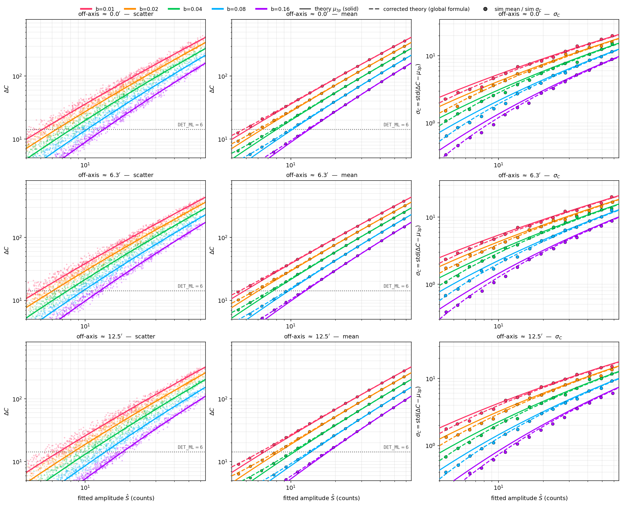
中心图展示位置趋势 低信号偏移和方差诊断 / The central figure shows location trends low signal shifts and variance diagnostics

Figure [fig:deltac-scatter-variance] is the central raw-data diagnostic for the matched experiment. It shows three facts needed by the distributional model: the pixel-sum location follows the dominant mean trend, the remaining low-signal location shift is smooth, and the Fisher-projected scale approaches the observed width at high signal. The rows show three representative detector radii and the colors show five backgrounds. The right column is the key variance diagnostic: the standard deviation is measured from $\Delta C-\mu_{3p}$ rather than from raw $\Delta C$, so gradients of the mean inside a bin do not masquerade as additional width. The dashed curves are descriptive fits to the same PN band-4 sample. The normalized $F(\mu_{3p})$ and $G(\mu_{3p})$ parameterization used for validation is introduced below.

Reference-fitter validation results

高信号闭合而低信号需要独立位置和宽度校正 / High signal closes while low signal needs separate location and width corrections

Table [tab:ref-fitter-validation] gives the two anchor regimes. At high signal ($\widehat S>20$), the standardized residual has mean 0.068 and width 0.977. Thus both the Asimov location and the projected scale close in the matched model. At $\widehat S<5$, the mean shifts upward to 0.922 Fisher units while the width contracts to 0.856. A low-count model must therefore correct location and scale separately.

Low-count location–scale kernel

原始标准化残差以理论位置和方差定义 / The raw standardized residual uses the theoretical location and variance

Define the raw normalized residual $$Z_0=\frac{\Delta C-\mu_{3p}}{\sqrt{V_{3p}}}.$$

紧凑函数将低计数残差的位置和宽度参数化 / Compact functions parameterize low count residual location and width

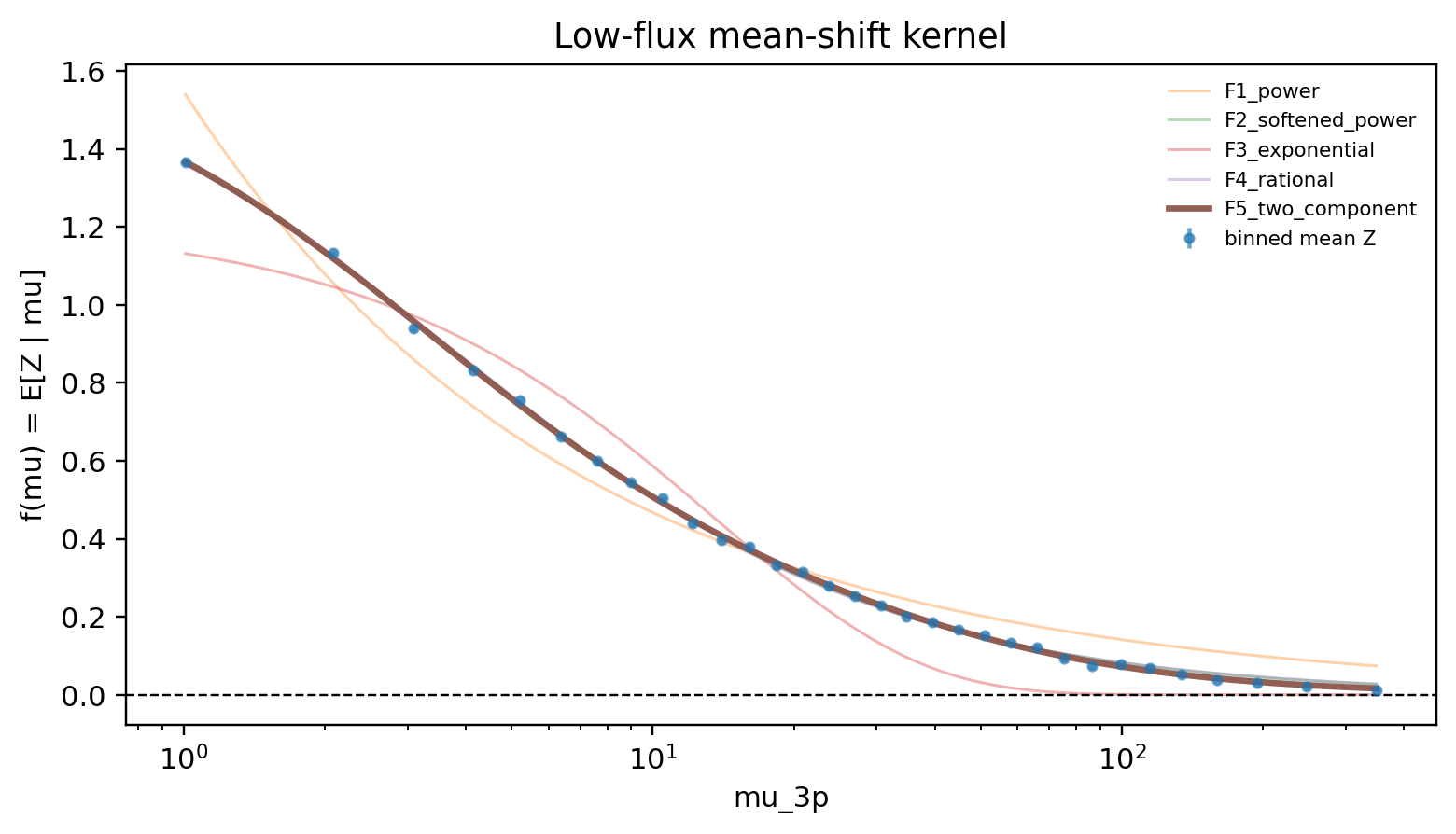
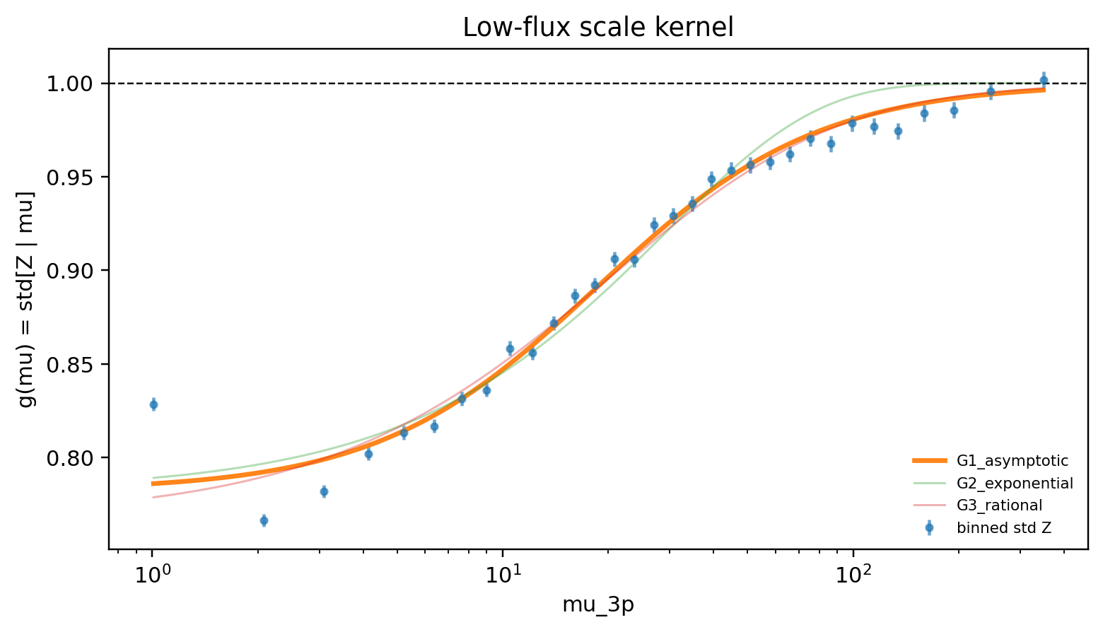
The low-count calibration estimates its location and scale as functions of the observable expected likelihood strength $\mu_{3p}$. The preferred compact functions are $$\begin{aligned} F(\mu) &= \frac{A_F}{1+(\mu/\mu_F)^{p_F}}, \\ G(\mu) &= 1-\frac{A_G}{1+(\mu/\mu_G)^{p_G}}, \label{eq:fg-kernel} \end{aligned}$$ with $$(A_F,\mu_F,p_F)=(1.7771,3.6904,0.9184)$$ and $$(A_G,\mu_G,p_G)=(0.21776,18.6075,1.3828).$$

校正后的条件位置和宽度由两个函数共同给出 / The two functions jointly give corrected conditional location and width

The conditional location and width are therefore $$\begin{aligned} \mu_{\Delta C}^\mathrm{corr} &=\mu_{3p}+\sqrt{V_{3p}}\,F(\mu_{3p}), \label{eq:mean-corr}\\ \sigma_{\Delta C}^\mathrm{corr} &=\sqrt{V_{3p}}\,G(\mu_{3p}). \label{eq:sigma-corr} \end{aligned}$$

两个经验函数拟合准确并在高信号回归 Fisher 极限 / Both empirical functions fit accurately and approach Fisher limits at high signal

The weighted RMSE values of $F$ and $G$ over 32 $\mu_{3p}$ bins are 0.0105 and 0.0107, respectively. Both functions approach their Fisher limits, $F\rightarrow0$ and $G\rightarrow1$, as $\mu_{3p}$ increases. The low-count location shift qualitatively recalls the empirical additive offset discussed by Stewart (2009), but here it is neither constant nor interpreted as the same correction.

Out-of-sample threshold validation

样本外阈值概率验证显示位置和宽度校正逐步改善 / Out of sample threshold validation shows stepwise gains from location and width corrections

The corrections were scored by threshold-passing probabilities at the fixed $\Delta C$ values corresponding to $\mathrm{DET\_ML}=6$, 8, and 10. No row was selected by observed $\mathrm{DET\_ML}$, $\Delta C$, or a residual. In the reconstructed realization-block split, the mean absolute error over the three thresholds falls from 0.013585 for the uncorrected Fisher kernel to 0.002428 after the location correction and to 0.001999 after both location and width corrections. The last value is close to the 0.001967 empirical-binned benchmark. Leave-one-position-out and leave-one-background-out tests give the same ordering (Table [tab:kernel-oos]).

宽度校正带来可复现的额外阈值概率改进 / The width correction provides a reproducible additional threshold probability gain

The improvement from the location correction is the largest, but the width term gives a reproducible further gain and nearly reaches the non-parametric cell benchmark. The result is a calibration of threshold-passing probabilities in the matched reference fitter. It is not evidence that transformed $\mathrm{DET\_ML}$ values are Gaussian, nor an injection-completeness measurement at fixed $S_\mathrm{true}$.

The mean correction does not determine the width

均值与宽度共享趋势但宽度仍需独立校正 / Mean and width share trends but width still needs an independent correction

Both $F$ and $G$ vary with $\mu_{3p}$, creating a visually strong pooled association. We tested whether an affine function of the fitted mean correction could replace the independently fitted $G(\mu_{3p})$. Under 17 whole-position folds, the independent and mean-linked width models give RMSE 0.040904 and 0.045494. Their ratio, 1.1122, misses the frozen 1.10 compression criterion. After the common $\mu_{3p}$ trend is removed, residual Spearman correlations between location and width are $-0.0465$ overall and $+0.0420$ for $5\leq\mu_{3p}\leq40$. The mean must be modeled to remove gradients before estimating a width, but the width requires its own correction function. This grouped test reuses the historical reference sample and is a model-discrimination result, not an independent confirmation data set.

Mechanism and configuration boundary

整数网格中位置重定位主导低计数均值偏移 / Position relocation dominates the low count mean shift on the integer grid

A targeted paired rerun saved oracle, amplitude-only, relocated-position, and full likelihood components for 96,000 fits across four detector positions. Among 49,193 clean rows with $\mu_{3p}<10$, amplitude optimization contributes $+0.838$ to the mean raw $\Delta C$ budget, whereas centroid relocation and position maximization contribute $+2.099$. Negative oracle/noise and fitted-conditioning terms cancel much of this gain, leaving a total fitted shift of $+0.692$. This supports a finite-position argmax interpretation in that integer-grid reference fitter, structurally analogous to look-elsewhere behavior (Gross & Vitells 2010). It does not establish the same component budget for continuous optimization or standalone emldetect.

配置内稳定性不代表经验系数跨配置通用 / Within configuration stability does not make empirical coefficients universal

Within the PN band-4 matched configuration, the compact $\mu_{3p}$ kernel leaves RMS location trends of 0.0073 across positions and 0.0377 across backgrounds. This within-configuration stability is useful but does not imply coefficient universality. PSF preparation, fitting mask, search domain, and optimizer are part of $k$ in Equation ([eq:master-kernel]); the cross-configuration test in Section 5 shows that changing them can change both the sign of $F_k$ and the scale $G_k$.

What the matched validation establishes

阈值范围验证支持匹配核但不支持普适精确尾部 / Threshold range validation supports the matched kernel not a universal exact tail

The high-signal closure alone would not justify threshold use: for the current PN band-4 configuration, $\mathrm{DET\_ML}=6$–10 lies mostly below $\widehat S=20$. The out-of-sample tests in Section 4.4 address this gap empirically for the matched reference fitter. They validate the compact location–scale kernel over the tested threshold range, but not an exact Gaussian tail law at arbitrarily small signal and not the behavior of another optimizer or PSF convention.

端到端注入校准绝对完备度而解析骨架保持连续依赖 / End to end injections calibrate absolute completeness while the analytical backbone retains continuous dependence

End-to-end fake-source injection remains the appropriate route for an absolute survey completeness calibration. It includes candidate generation, source confusion, background-map construction, and every pipeline cut, as in modern simulation-calibrated survey analyses (Brunner et al. 2022; Liu et al. 2022). The purpose of the analytical backbone is different. Equations ([eq:mu3p]) and ([eq:var3p]) carry the continuous dependence on background, PSF, and mask. A matched simulation then calibrates two dimensionless functions, $F_k$ and $G_k$, rather than tabulating a dense distribution at every position and flux. Section 5 tests how much additional state is needed when the fitter is changed to standalone emldetect.

Pipeline-Specific Calibration and Transfer Boundary

匹配参考拟合器仍需独立管线校准且不可跨配置转移 / The matched reference fitter still needs standalone calibration and cannot transfer across configurations

The matched reference fitter isolates the statistical theory, but SAS emldetect has a different optimizer, internally rendered PSF, search surface, and mask convention. This section retains the historical PN band-4 standalone experiment as a case study of the required extra calibration. Its first result is a position-dependent calibration of the mean crossing; it is not an absolute completeness measurement. The second result is a transfer test showing that neither this calibration nor the reference-fitter $F$ and $G$ coefficients can be assumed to hold for another camera/band/search configuration.

PN band-4 mean residual calibration

原始理论给出阈值位置但在阈值带存在位置依赖误差 / Raw theory locates thresholds but has position dependent errors in the threshold band

The raw theory supplies the Asimov location $$\mu_{3p}(\widehat S,b,\mathrm{psf},\mathrm{mask}) \simeq E[\Delta C\mid\widehat S,b,\mathrm{psf},\mathrm{mask}]$$ If standalone emldetect exactly matched the same model, the threshold limit could be found from $$\mu_{3p}(S_{\mathrm{lim}},b,\mathrm{psf},\mathrm{mask}) = \Delta C_{\mathrm{th}}$$ In practice, this uncalibrated-theory baseline is only a borderline approximation in the threshold band. In the validation, it has maximum $S_\mathrm{lim}$ errors of 19.9% at $\mathrm{DET\_ML}=6$, 15.6% at $\mathrm{DET\_ML}=8$, and 13.3% at $\mathrm{DET\_ML}=10$. The error is position-dependent rather than a single scalar offset.

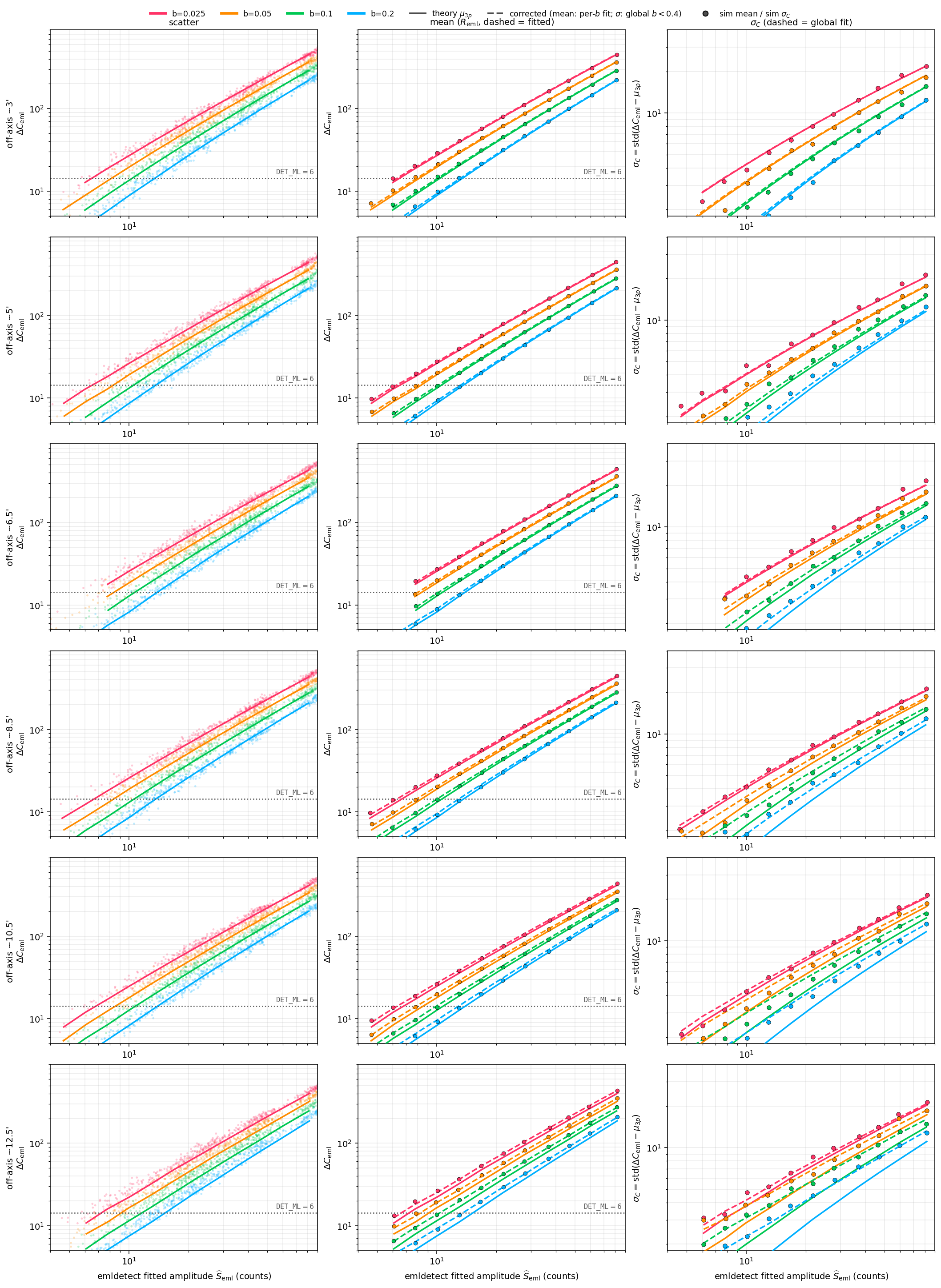
独立管线相对参考理论存在位置依赖残差 / The standalone pipeline has a position dependent residual relative to reference theory

Figure [fig:emldetect-scatter-variance] is the central diagnostic for the operational standalone-emldetect chain. It is deliberately parallel to Figure [fig:deltac-scatter-variance]: the same observable-conditioned structure remains visible, but the standalone pipeline introduces a position-dependent residual relative to the reference-fitter theory. This is the visual reason that the final calibration is not the raw analytic equation, but the analytic equation plus an empirical $R_\mathrm{eml}$ calibration.

定义独立拟合器相对理论的残差 / Defines the standalone fitter residual relative to theory

We therefore define the standalone emldetect residual

$$R_{\mathrm{eml}} = \Delta C_{\mathrm{eml}} - \mu_{3p}(\widehat{S}_{\mathrm{eml}},b,\mathrm{psf},\mathrm{mask}) \label{eq:reml}$$

说明独立输出量并建立校正阈值方程 / Explains standalone outputs and introduces the calibrated threshold equation

Here $\Delta C_\mathrm{eml}$ is the standalone emldetect Cash improvement converted with the single-image $\nu=3$ convention, and $\widehat{S}_\mathrm{eml}$ is the fitted emldetect source amplitude. The calibrated threshold equation is

$$\mu_{3p}(S_{\mathrm{lim}},b,\mathrm{psf},\mathrm{mask}) = \Delta C_{\mathrm{th}} - \widehat{R}_{\mathrm{eml}} \label{eq:sensitivity-limit}$$

残差符号决定理论阈值与源强的调整方向 / Residual sign determines how the theoretical threshold and source strength shift

The sign follows directly from the residual definition. If $\widehat{R}_\mathrm{eml}>0$, standalone emldetect produces larger $\Delta C$ than the raw theory at the same fitted source strength, so the theoretical threshold needed for the sensitivity limit is lower. If $\widehat{R}_\mathrm{eml}<0$, the required source amplitude is higher.

配对模拟以预测参考量选取阈值带并评估背景转移 / Paired simulations select the threshold band by reference prediction and assess background transfer

The calibration uses paired fake-source simulations in which each realization is analyzed both by the reference fitter and by standalone SAS emldetect. The current calibration grid has 14 PN band-4 calibration positions after excluding the edge-affected case. The target threshold band is defined in $\Delta C$ space using the threshold conversions of Equation ([eq:detml-inverse]). Rows are selected by the reference-theory prediction: $$\mu_{3p,\mathrm{ref}} \in [\Delta C_{\mathrm{ML6}}, \Delta C_{\mathrm{ML10}}]$$ This is important: the threshold sample is not selected by observed $\mathrm{DET\_ML}_\mathrm{eml}$ or by observed $\Delta C_\mathrm{eml}$, because those quantities carry the stochastic fluctuation and implementation residual we are trying to calibrate. The selection is based on the predicted/reference $\Delta C$ in the observable-conditioned theory. The baseline calibration grid is built at $b = 0.04\,\mathrm{counts\,pixel^{-1}}$; background transfer to $b=0.02$ and $b=0.08\,\mathrm{counts\,pixel^{-1}}$ is included in the uncertainty budget below.

按位置估计残差并比较两种插值校准方案 / Residuals are estimated by position using two interpolation calibration schemes

The residual $\widehat{R}_\mathrm{eml}$ is estimated at each detector position from the threshold-band simulation sample. We compare a 2D interpolation over off-axis radius and a sector-coded calibration coordinate with nearest-position assignment. The sector code has four quadrant values; it is an interpolation label, not a physical detector azimuth and not a portable PSF descriptor.

Leave-one-position-out mean-crossing interpolation

留一位置验证预测内部阈值映射而非绝对完备度 / Leave one position validation tests internal threshold mapping not absolute completeness

Validation uses leave-one-position-out cross-validation: each position is held out, the calibration is built from the remaining positions, and the predicted $S_\mathrm{lim}$ is compared to the held-out position’s internally calibrated reference limit. This held-out reference limit, $S_\mathrm{ref}$, is defined using the same reference fitter that is used throughout Section 4: for each simulated source strength, the median $\Delta C_\mathrm{fit}$ across repetitions is computed, a smooth interpolating spline is fitted to the median $\Delta C_\mathrm{fit}$ versus source-strength curve, and $S_\mathrm{ref}$ is defined as the exact root where the spline crosses $\Delta C_\mathrm{threshold}$. No information from the held-out position is permitted to leak into the $\widehat{R}_\mathrm{eml}$ interpolation model, ensuring a strict out-of-sample prediction test. We emphasize that this cross-validation tests the calibration’s ability to self-consistently interpolate the pipeline’s own threshold mapping across the calibration grid; it is not an absolute astrophysical validation against independent observational data or against injection-recovery detection fractions. Such absolute validation, for example comparing the predicted $S_\mathrm{lim}$ against an injection-recovery 50% completeness flux from dense fake-source injection at representative positions, is a necessary future step for production use. The reported error is

$$|S_{\mathrm{lim,pred}} - S_{\mathrm{ref}}| / S_{\mathrm{ref}}$$

阈值误差验证量化插值范围与背景转移的表现 / Threshold errors quantify interpolation coverage and background transfer performance

Table [tab:unified-validation] summarizes this conditional interpolation estimand. At $\mathrm{DET\_ML}=6$, the preferred 2D interpolation yields a median error of 4.1% and a maximum error of 11.0% for positions inside the calibration hull (10 of 14 held-out positions); the nearest-calibration-position assignment covers all 14 positions with a maximum error of 17.2%. Background transfer from $b=0.04\,\mathrm{counts\,pixel^{-1}}$ to the range $b=0.02$–$0.08\,\mathrm{counts\,pixel^{-1}}$ adds at most 5.7% error in $S_\mathrm{lim}$ at $\mathrm{DET\_ML}=6$. Both errors decrease at higher thresholds.

未校正理论和全局修正均不能提供绝对灵敏度 / Uncorrected theory and global correction do not provide absolute sensitivity

The uncalibrated theory has a maximum $S_\mathrm{lim}$ error of 19.9% at $\mathrm{DET\_ML}=6$ (7.2% median), making it only borderline as a standalone approximation at the most stringent threshold. A global scalar correction fails at $\mathrm{DET\_ML}=6$ (maximum error 21.6%), confirming that the residual is position dependent. The 2D interpolation is preferred inside the calibration hull; nearest-position assignment is the tested fallback for the 14-position sample. These percentages are interpolation errors relative to an internally defined crossing. They are not completeness or absolute sensitivity errors.

Standalone width is a separate calibration target

独立宽度需单独校准且现有抖动模型尚未获验证 / Standalone width needs separate calibration and the jitter model remains unvalidated

The mean-crossing result does not calibrate the standalone width. A historical paired sample of 20,855 rows in 148 cells was analyzed with 14 whole-position folds. An affine relation between reference and standalone $\Delta C$ describes the mean, but propagating its slope alone underpredicts the width: the held-out log-width RMSE is 0.190244 and the geometric observed-to-predicted ratio is 1.186469. Adding one constant jitter term in quadrature, $$\sigma_\mathrm{eml}^2=a^2\sigma_\mathrm{ref}^2+\tau^2, \label{eq:eml-jitter}$$ with median training-fold $\tau=1.837\,\Delta C$, improves those values to 0.134238 and 1.040060. Two held-out positions remain substantially miscalibrated. Equation ([eq:eml-jitter]) is therefore a development candidate for that historical data set, not a validated standalone or cross-camera width law.

M1/M2 cross-configuration falsification

大规模跨相机测试显示位置和宽度都需配置校正 / Large cross camera tests show location and width both need configuration correction

A larger standalone development test assembled 16,308,000 M1/M2 rows. Its homogeneous primary subset contains M1 band 4, M2 band 1, and M2 band 4, with cells defined in fitted-observable space near theoretical $\mathrm{DET\_ML}=6$–10. The coefficient-free analytic backbone gives a row-weighted mean residual of $-0.93749$ and a median width ratio $\sigma_\mathrm{obs}/\sqrt{V_{3p}}=0.83715$. Exact row-mixture passing-fraction MAE values are 0.06290, 0.10795, and 0.06340 at $\mathrm{DET\_ML}=6$, 8, and 10. Thus both location and width require a standalone configuration correction.

冻结的参考核不能作为联合规律跨配置转移 / The frozen reference kernel cannot transfer across configurations as a joint law

The frozen PN band-4 reference kernel does not transfer as a combined law. Its positive location correction has the wrong sign: in whole-configuration validation, mean RMSE worsens from 1.21980 for the uncorrected baseline to 2.02904 after transfer. The width component alone improves width-ratio RMSE from 0.21518 to 0.15634, but this partial similarity does not rescue the joint kernel. A newly fitted shared transition reaches mean and width-ratio RMSE of 0.96166 and 0.15273; none of the preregistered injection-PSF feature additions passes both configuration and coordinate gates.

负结果否定通用系数但不否定位置尺度分解 / The negative result rejects universal coefficients not the location scale decomposition

This negative result rejects universal coefficients, not the location–scale decomposition. The stored injection template is not the same object as the internal ELLBETA PSF/search surface used by emldetect, so the test does not show that PSF information is irrelevant or that a fitter-state-conditioned calibration is impossible. No multiband PN outcome is used here. A one-realization-per-cell three-camera execution has established technical feasibility only and cannot estimate a conditional width.

Threshold-Crossing and Population-Inference Consequences

条件矩支持将检测阈值视为概率穿越事件 / Conditional moments turn detection thresholds into probabilistic crossing events

Once both conditional moments are available, a detection threshold can be treated as a crossing event rather than as a deterministic equality. This section gives two mathematical consequences. A conventional $\mathrm{DET\_ML}$-selected catalog can be interpreted backward in fitted-amplitude space after supplying a prior, or a calibrated kernel can be used forward to define fitted-amplitude percentile crossings. These are consequences of a conditional kernel, not claims that the historical standalone case study or an official XMM catalog already has a validated selection function.

本文的 S 是拟合振幅而非注入本征流量 / Here S denotes fitted amplitude rather than injected intrinsic flux

Here $S$ denotes the source-amplitude coordinate used by the observable-conditioned theory, consistent with the fitted-amplitude convention used throughout this work. It is not an intrinsic injected flux.

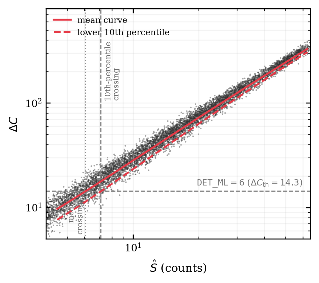
图示将阈值核分别用于反演解释和前向切割 / The figure shows inverse interpretation and forward cuts from the threshold kernel

Figure 1 gives the visual version of the construction. A traditional $\mathrm{DET\_ML}$ threshold is a horizontal cut in $\Delta C$ space. Reading the conditional distribution backward from that cut gives the fitted-amplitude distribution of a traditional threshold-selected catalog, once a source-count prior is specified. Reading it forward gives percentile crossings: the usual sensitivity map is the mean crossing, while a lower-percentile crossing defines a more conservative fitted-amplitude threshold-crossing cut.

The forward kernel in $\Delta C$ space

操作 DET ML 阈值先转换为三参数 Delta C 阈值 / Operational DET ML thresholds are first converted to three parameter Delta C thresholds

For each detector position, the operational $\mathrm{DET\_ML}$ threshold is first converted to the corresponding single-image three-parameter $\Delta C$ threshold. For example, $\mathrm{DET\_ML}=6$ corresponds to $\Delta C_\mathrm{th}=14.3$ under the $\nu=3$ convention. The distributional calculation is then carried out in $\Delta C$ space; $\mathrm{DET\_ML}$ remains only the final operational threshold scale.

每个配置以校正位置和宽度函数定义阈值曲线 / Each configuration defines threshold curves with calibrated location and width functions

For a configuration $k$ with calibrated location and width functions, define

$$\begin{aligned} \Delta C_\mathrm{mean}^{(k)}(S,x,b) &=\mu_{3p}(S,b,\mathcal{P}_x,\mathcal{M}_x) +\sqrt{V_{3p}(S,b,\mathcal{P}_x,\mathcal{M}_x)}\, F_k(\mu_{3p}), \label{eq:mean-threshold-curve} \\ \sigma_C^{(k)}(S,x,b) &=\sqrt{V_{3p}(S,b,\mathcal{P}_x,\mathcal{M}_x)}\, G_k(\mu_{3p}). \label{eq:width-threshold-curve} \end{aligned}$$

高斯残差近似将局部核写成正态分布 / The Gaussian residual approximation summarizes the local kernel as a normal distribution

With the Gaussian residual approximation, the local kernel is summarized as

$$p(\Delta C\mid S,x,b) \simeq \mathcal{N}\!\left[ \Delta C_\mathrm{mean}^{(k)}(S,x,b),\, \{\sigma_C^{(k)}(S,x,b)\}^2 \right], \label{eq:deltac-forward-kernel}$$

and the corresponding $p$th percentile curve is

$$\Delta C_{p}(S,x,b) \simeq \Delta C_\mathrm{mean}^{(k)}(S,x,b) +z_p\,\sigma_C^{(k)}(S,x,b), \label{eq:deltac-percentile-curve}$$

where $z_p$ is the standard-normal quantile. The percentile construction requires, in addition to the calibrated mean residual, a calibrated threshold-band scatter model $\sigma_C$ in $\Delta C$ space. Thus $\Delta C_{50}\simeq \Delta C_\mathrm{mean}^{(k)}$, $\Delta C_{16}\simeq \Delta C_\mathrm{mean}^{(k)}-\sigma_C^{(k)}$, $\Delta C_{10}\simeq \Delta C_\mathrm{mean}^{(k)}-1.282\,\sigma_C^{(k)}$, and $\Delta C_{2.3}\simeq \Delta C_\mathrm{mean}^{(k)}-2\,\sigma_C^{(k)}$.

匹配参考核已验证而独立管线宽度仍待验证 / The matched reference kernel is validated while standalone width remains unvalidated

For the matched PN band-4 reference fitter, $F_k$ and $G_k$ are the functions validated in Section 4. The historical standalone experiment calibrates a mean residual $\widehat R_\mathrm{eml}(x)$, so its mean can be written $\mu_{3p}+\widehat R_\mathrm{eml}$ within that case study. It does not yet supply a deployable $G_k$ across all positions. Consequently, the lower-percentile formulas are demonstrated for the matched kernel; their standalone use remains conditional on a new width and tail validation.

Application I: interpreting traditional $\mathrm{DET\_ML}$-selected catalogs

应用一以观测阈值目录和前向核解释拟合振幅 / Application one interprets observed threshold catalogs through the forward kernel

The first application keeps the traditional catalog definition. A source is selected by an observed detection statistic, for example $\mathrm{DET\_ML}>T$, equivalently $\Delta C>\Delta C_\mathrm{th}$. The new ingredient is that the catalog threshold can now be interpreted through the forward kernel in Equation ([eq:deltac-forward-kernel]).

单源的拟合振幅后验由核和先验相乘得到 / A single source fitted amplitude posterior combines the kernel and prior

For a source with a measured value $\Delta C_\mathrm{obs}$, the fitted-amplitude posterior in catalog space is

$$p(S\mid \Delta C_\mathrm{obs},x,b) \propto p(\Delta C_\mathrm{obs}\mid S,x,b)\,\pi(S), \label{eq:posterior-single-source}$$

where $\pi(S)$ is a source-count prior expressed in the fitted-amplitude coordinate. For a threshold-selected ensemble, the analogous expression is

$$p(S\mid \Delta C>\Delta C_\mathrm{th},x,b) \propto P(\Delta C>\Delta C_\mathrm{th}\mid S,x,b)\,\pi(S), \label{eq:posterior-threshold-selected}$$

with

$$P(\Delta C>\Delta C_\mathrm{th}\mid S,x,b) = \int_{\Delta C_\mathrm{th}}^\infty p(\Delta C\mid S,x,b)\,d\Delta C . \label{eq:threshold-passing-probability}$$

越阈概率加先验解释目录并引入 Eddington 偏差 / Threshold probability plus a prior interprets catalogs and introduces Eddington bias

Under the Gaussian residual approximation, this passing probability is a normal survival function evaluated in $\Delta C$ space. This route does not replace the traditional $\mathrm{DET\_ML}$ threshold. Instead, it adds the missing likelihood layer needed to interpret the fitted-amplitude distribution of a $\mathrm{DET\_ML}$-selected catalog. This is also the point at which Eddington bias enters: the noisy threshold statistic must be combined with a source-count prior, especially when the underlying $dN/dS$ is steep (Eddington 1913; Georgakakis et al. 2008; Wang 2004). A specified $\mathrm{DET\_ML}$ value or threshold therefore does not by itself define a flux distribution; it defines a likelihood factor in $\Delta C$ space. To obtain $p(S\mid \Delta C_\mathrm{obs})$ or $p(S\mid \Delta C>\Delta C_\mathrm{th})$, one must combine that likelihood with a source-count prior, for example a power-law $dN/dS$ slope or index expressed in the fitted-amplitude coordinate. Because this is an inverse problem, it necessarily depends on the population prior. If the desired prior is an intrinsic $dN/dS_\mathrm{true}$ rather than a prior in fitted catalog amplitude, an additional measurement model connecting $S_\mathrm{true}$ to the fitted amplitude $S$ is required.

目录有效面积是概率加权而非硬幅度极限 / Catalog effective area is probability weighted rather than a hard amplitude limit

The corresponding fitted-amplitude effective area is probabilistic rather than a step function derived from one limiting amplitude. At a given pixel $j$, detecting a source with fitted amplitude $S$ has the catalog-space density

$$q_j(S) \propto P(\Delta C>\Delta C_\mathrm{th}\mid S,x_j,b_j)\,\pi(S), \label{eq:pixel-detected-amplitude-density}$$

up to normalization over the fitted-amplitude coordinate. Thus the traditional threshold catalog assigns a probability to detected amplitudes at each pixel, rather than a single deterministic limiting amplitude. The catalog-space effective area at fitted amplitude $S$ is

$$\Omega_\mathrm{th}(S) = \sum_j \Omega_j\, P(\Delta C>\Delta C_\mathrm{th}\mid S,x_j,b_j), \label{eq:traditional-probabilistic-sky-coverage}$$

where $j$ indexes sky or detector pixels. If the goal is the expected number of detected fitted amplitudes in an interval $A$, the same probability-weighted area is combined with the source-count prior,

$$N_\mathrm{det}(A) \propto \int_A \Omega_\mathrm{th}(S)\,\pi(S)\,dS . \label{eq:traditional-detected-amplitude-distribution}$$

目录空间面积不是真实流量选择函数且需联合模型 / Catalog space area is not a true flux selection function and needs a joint model

Equation ([eq:traditional-probabilistic-sky-coverage]) is not a true-flux selection function. The latter requires the joint measurement model that the observable-conditioned kernel deliberately does not supply. For the idealized selection event $\Delta C>\Delta C_\mathrm{th}$ alone, the true-flux effective area would be $$\Omega_\mathrm{true}(S_\mathrm{true}) =\sum_j\Omega_j \iint_{\Delta C>\Delta C_\mathrm{th}} p(\Delta C,\widehat S\mid S_\mathrm{true},x_j,b_j) \,d\Delta C\,d\widehat S. \label{eq:true-flux-sky-coverage}$$ Additional candidate-generation and catalog-inclusion rules enlarge the joint state and replace this integration domain by the full selection event. A factorization into $p(\Delta C\mid\widehat S,x_j,b_j) p(\widehat S\mid S_\mathrm{true},x_j,b_j)$ is useful only after its conditional-independence and transport assumptions have been checked in matched injection simulations.

应用一按检测振幅分布而应用二按目标穿越概率定义 / Application one follows detected amplitudes while application two fixes a crossing probability

This is the sense in which the catalog-space effective area for Application I follows the probability distribution of detected fitted amplitudes, whereas the percentile-cut construction below starts from a chosen fitted-amplitude threshold-crossing probability.

Application II: fitted-amplitude percentile cuts

应用二固定拟合振幅并前向计算越阈概率无需源计数先验 / Application two fixes fitted amplitude and computes crossing probability without a source count prior

The second application uses the same kernel in the forward direction. Instead of starting from a noisy $\mathrm{DET\_ML}$-selected sample and asking what fitted amplitudes it contains, one asks what fitted amplitude is required for a specified fraction of realizations to exceed the detection threshold. This map-construction step fixes $S$ and evaluates $P(\Delta C>\Delta C_\mathrm{th}\mid S,x,b)$, so no $dN/dS$ slope or source-count index is required.

均值曲线穿越恢复常用灵敏度图定义 / The mean curve crossing recovers the usual sensitivity map definition

The usual sensitivity-map calculation is recovered as the mean-curve crossing

$$\Delta C_\mathrm{mean}^{(k)}(S,x,b)=\Delta C_\mathrm{th}. \label{eq:mean-curve-crossing}$$

均值穿越只在高斯近似下对应百分之五十且非注入完备度 / The mean crossing is 50 percent only under Gaussian residuals and is not injection completeness

Under a symmetric Gaussian residual approximation, this is also the 50th-percentile threshold-crossing point. We avoid calling it an empirical 50% completeness flux, because injection-recovery completeness is usually defined as $P(\mathrm{detected}\mid S_\mathrm{true})$ in the injected-flux coordinate.

更保守切割由低百分位阈值曲线的穿越确定 / More conservative cuts solve threshold crossings with lower percentile curves

More conservative fitted-amplitude cuts are obtained by solving the threshold equation with lower percentile curves,

$$\Delta C_p^{(k)}(S,x,b)=\Delta C_\mathrm{th}, \label{eq:percentile-threshold-crossing}$$

with $p<50$. The direction is important. Requiring 90% of realizations at a given fitted amplitude to exceed the threshold uses the lower 10th percentile, not the upper 90th percentile:

$$\Delta C_{10}^{(k)}(S,x,b)=\Delta C_\mathrm{th}.$$

下二倍标准差包络近似要求百分之九十七点七穿越 / A lower two standard deviation envelope requires about 97 point 7 percent crossing

Similarly, using the $\mu-2\sigma$ lower envelope corresponds to an approximately 97.7% threshold-crossing criterion under the Gaussian approximation. Table [tab:threshold-crossing-terms] summarizes the terminology used here.

Fitted-amplitude effective area for threshold crossings

逐像素穿越规则形成拟合振幅灵敏度图及有效面积 / Pixelwise crossing rules yield fitted amplitude sensitivity maps and effective area

Applying the same crossing rule to every detector pixel produces a family of fitted-amplitude sensitivity maps: a mean-threshold map, an 84% threshold-crossing map from the lower 16th percentile, a 90% threshold-crossing map from the lower 10th percentile, and so on. Each map can be converted into a fitted-amplitude effective-area curve by counting the sky area over which the local limiting amplitude is below a trial fitted amplitude,

$$\Omega_{p,\rm fit}(S) = \sum_j \Omega_j\, I\!\left[S_\mathrm{lim}^{(p)}(j) \le S\right],$$

where $j$ indexes sky or detector pixels and $p$ denotes the percentile curve used in Equation ([eq:percentile-threshold-crossing]). This threshold-crossing effective-area calculation is an instrumental, catalog-space quantity in the same fitted-amplitude coordinate used by the observable-conditioned theory: it depends on the local background, PSF, mask, threshold, and residual calibration, but it does not require an assumed $dN/dS$ slope. It should not be relabeled as $\Omega(S_\mathrm{true})$; Equation ([eq:true-flux-sky-coverage]) is needed for that quantity. A source-count model is needed in subsequent population inference.

Relation between the two uses and Eddington bias

同一条件核支撑反向 Eddington 建模和前向概率问题 / The same conditional kernel supports inverse Eddington modeling and forward probability questions

Both applications come from the same conditional distribution $p(\Delta C\mid S,x,b)$, but they answer different questions. Application I is backward: it starts from an observed $\mathrm{DET\_ML}$ value or a $\mathrm{DET\_ML}$-selected catalog and infers the fitted-amplitude distribution. This is the natural setting for Eddington-bias modeling, because the asymmetry near a detection threshold is produced by combining the noisy threshold statistic with a steep source-count prior.

应用二构造概率明确的子样本但不消除总体偏差 / Application two builds a probability defined subsample but does not remove population bias

Application II is forward: it starts from a fitted amplitude and asks for the probability of crossing the $\mathrm{DET\_ML}$ threshold. This does not remove population-level Eddington bias from a luminosity-function inference, but it allows one to construct an instrumental catalog-space subsample with an explicitly stated threshold-crossing probability. In this sense, the percentile sensitivity map is a catalog-construction tool, whereas the threshold-selected posterior is a catalog-interpretation tool.

真实流量去偏需要联合测量模型而条件核仅为其中一项 / True flux deboosting needs a joint measurement model and the conditional kernel is one factor

True-flux deboosting is a larger problem. It requires $p(\widehat S,\Delta C\mid S_\mathrm{true},x,b)$, a prior on $S_\mathrm{true}$, and normalization by the same selection event used to form the catalog. The conditional $\Delta C\mid\widehat S$ kernel is one factor in that calculation, not a complete Eddington correction by itself.

Validation requirements and limitations

低百分位独立图需全新通过率验证而官方目录需端到端检验 / Lower percentile standalone maps need new passing validation and official catalogs need end to end tests

Section 4 validates threshold-passing probabilities for the matched reference fitter. Section 5 measures only the interpolation error of the historical standalone mean crossing: at $\mathrm{DET\_ML}=6$, the maximum is 11.0% inside the calibration hull and 17.2% for nearest-position assignment across all 14 held-out positions. The standalone width and tails are not closed. Before a lower-percentile standalone map is used, predicted passing probabilities must be compared with empirical passing fractions in new whole-position simulations. An official catalog adds candidate-generation and inclusion rules that require a separate end-to-end selection test.

本应用是阈值解释框架而真实流量函数仍依赖注入恢复 / This application is a threshold interpretation framework while true flux selection needs injection recovery

Thus the application presented here is a distributional framework for threshold interpretation and fitted-amplitude threshold crossing. Full injection-recovery simulations remain the validation standard for a true-flux selection function in complex survey fields.

发布后将通过持久 Zenodo 档案提供复现材料 / Reproduction materials will be released through a persistent Zenodo archive

The calibration grid, cross-validation tables, figure-generation scripts, configuration files, and minimal scripts reproducing key validation results will be made available upon publication via a persistent Zenodo archive.

Scope and Limitations

解析分解可移植 经验函数需要匹配标定 / The analytic decomposition is portable but empirical functions require matched calibration

The evidence tiers are summarized in Table [tab:evidence-tiers]. The analytical decomposition is the portable result. The numerical $F_k$ and $G_k$ functions are attached to a particular effective PSF, mask, search domain, and fitter. Changing camera or energy band changes the PSF, but changing the pipeline can also change the internal PSF raster and optimization state even when the stored injection template is held fixed. Quantitative transfer therefore requires matched calibration rather than a camera label alone.

验证仅覆盖特定单图像点源拟合及有限背景范围 / Validation covers only specific single image point source fits and a limited background range

The matched simulations are single-image, isolated point-source fits on a locally specified background. Extended sources, crowded fields, multi-image likelihoods, merged observations, background-estimation uncertainty, and a different number of fitted degrees of freedom are outside the derivation as tested. The reference kernel is validated in PN band 4. The historical standalone mean grid covers $b=0.02$–$0.08\,\mathrm{counts\,pixel^{-1}}$ only; its sector coordinate is not a physical PSF parameter. The M1/M2 experiment is a strong negative transfer test, but the exact internally rendered ELLBETA fit/search object was not saved, so it cannot determine which missing fitter-state variable would restore portability.

目录阈值样本不能独立确定弱源条件宽度 / Catalog threshold samples cannot independently determine weak source conditional width

No catalog-selected sample is used as core evidence for the weak-source kernel. Near a catalog threshold, the unselected parent distribution is unknown; a likelihood-selected catalog cannot by itself identify the conditional width of the missing sources. Official catalog selection also includes stacking, confusion, vignetting, background-map variation, and joint multi-band decisions. End-to-end simulations used by other survey pipelines illustrate why these effects are normally calibrated as a complete system (Brunner et al. 2022; Evans et al. 2024; Liu et al. 2022).

有效面积仍在拟合振幅坐标 真流量推断需要联合模型 / Effective area remains in fitted amplitude coordinates and true flux inference needs a joint model

Finally, all Section 6 effective-area curves before Equation ([eq:true-flux-sky-coverage]) live in the fitted-amplitude coordinate. Population-level Eddington correction and true-flux sky coverage require a source prior and a joint measurement model connecting $S_\mathrm{true}$, $\widehat S$, and $\Delta C$.

Conclusions

Fisher 投影方差给出条件 Delta C 宽度并需低计数修正 / Fisher projected variance gives conditional Delta C width and needs low count correction

The main analytical result is the leading Fisher approximation to the conditional width $$\sigma_{\Delta C} \simeq \sqrt{4\left[ \sum_i M_i\mu_i\ln^2(\mu_i/b_i)-g^TI^{-1}g \right]}.$$ The Fisher projection removes the amplitude and two position score directions absorbed by the fit. It is evaluated from fitted observables, the pixelized PSF, background, and mask. The companion $\mu_{3p}$ expression extends the amplitude-only analytical Cash-sensitivity calculation of Stewart (2009); Stewart (2006) provides earlier matched-filter sensitivity context. The variance is the element that turns a deterministic threshold curve into a distribution, with $G_k$ supplying the empirically measured low-count width correction.

匹配 PN 波段四验证位置尺度核及独立宽度校正 / Matched PN band four validation supports the location scale kernel and independent width correction

In the matched PN band-4 reference fitter, 266,837 high-signal fits give a standardized residual mean of 0.068 and width of 0.977. At low signal, the empirical location–scale kernel $$\Delta C\simeq \mathcal{N}\!\left[ \mu_{3p}+\sqrt{V_{3p}}F(\mu_{3p}), V_{3p}G^2(\mu_{3p}) \right]$$ describes 810,987 clean fits. In realization-block validation, the mean passing-fraction error over $\mathrm{DET\_ML}=6$, 8, and 10 decreases from 0.013585 for raw Fisher theory to 0.001999 after both corrections, close to the 0.001967 empirical-bin benchmark. The width improvement is smaller than the location improvement but reproducible. A grouped test also rejects replacing $G$ by a function inferred from $F$ alone. The mean centers the residual and removes cell gradients; it does not determine the conditional width.

独立 emldetect 校准仅限管线且系数不能跨相机转移 / Standalone emldetect calibration is pipeline specific and coefficients do not transfer across cameras

Standalone emldetect remains scientifically useful in this framework, but as a pipeline-specific layer. The historical PN band-4 experiment quantifies interpolation of an internally defined mean crossing. Its 11–17% errors are not completeness errors, and its width is not closed. The M1/M2 development experiment provides the complementary boundary: unchanged PN coefficients fail to transfer. In the primary theoretical-$\mathrm{DET\_ML}=6$–10 development cells, the row-weighted location residual is about $-0.94\,\Delta C$ and the median observed-to-Fisher width ratio is about 0.84. The reusable result is therefore the analytical location–scale architecture, not a universal coefficient table.

匹配核定义拟合振幅越阈概率 真流量修正仍需完整联合模型 / The matched kernel defines fitted amplitude crossings while true flux correction still needs a full joint model

The calibrated matched kernel defines fitted-amplitude threshold-crossing probabilities and a fitted-amplitude effective area. Backward catalog interpretation requires a prior. True-flux completeness and Eddington correction additionally require the joint measurement model $p(\Delta C,\widehat S\mid S_\mathrm{true},x,b)$ and the catalog’s full selection normalization. These boundaries preserve the practical value of the new $\sigma_{\Delta C}$ form while keeping its empirical coefficients tied to the PSF/search/fitter configuration in which they were measured.

Data and Code Availability

复现材料和机器可读标定表将在发表时持久归档 / Reproduction materials and machine readable calibration tables will be persistently archived upon publication

The calibration grid, cross-validation tables, figure-generation scripts, SAS configuration files, and minimal scripts reproducing key validation results (including the exact commands, random seeds, PSF parameters, and emldetect invocation flags) will be deposited in a persistent archive upon publication. The DOI and license will be inserted before submission. Machine-readable calibration tables and the code used to generate the figures are maintained with the project artifacts during review.

Author Contributions

作者贡献暂列主要工作并待全体作者确认角色 / Author contributions list primary work and await all author role confirmation

R.H. developed the statistical model, simulations, analysis code, and initial manuscript. Draft note: coauthor roles will be completed using the CRediT taxonomy after all authors approve the submission version.

Competing Interests

利益冲突声明将在投稿前由全体作者确认 / The competing interests declaration will be confirmed by all authors before submission

Draft note: the competing-interest declaration will be confirmed by all authors before submission.

Funding

本研究获国家自然科学基金支持且资助编号待确认 / This work has national science foundation support and grant identifiers await confirmation

This work acknowledges support from the National Natural Science Foundation of China. Draft note: grant identifiers will be added after author confirmation.

Ethics Statement

研究仅用模拟和档案标定产品 不涉及受试对象或个人数据 / The study uses only simulations and archival calibration products with no subjects or personal data

This study uses numerical simulations and archival calibration products; it involves no human participants, animals, or personally identifiable data.

AI-Assistance Disclosure

人工智能协助声明将按目标期刊政策在投稿前定稿 / The AI assistance disclosure will be finalized under target journal policy before submission

Draft note: a disclosure consistent with the policy of the selected journal will be finalized before submission.

Diagnostic role of injected source strength

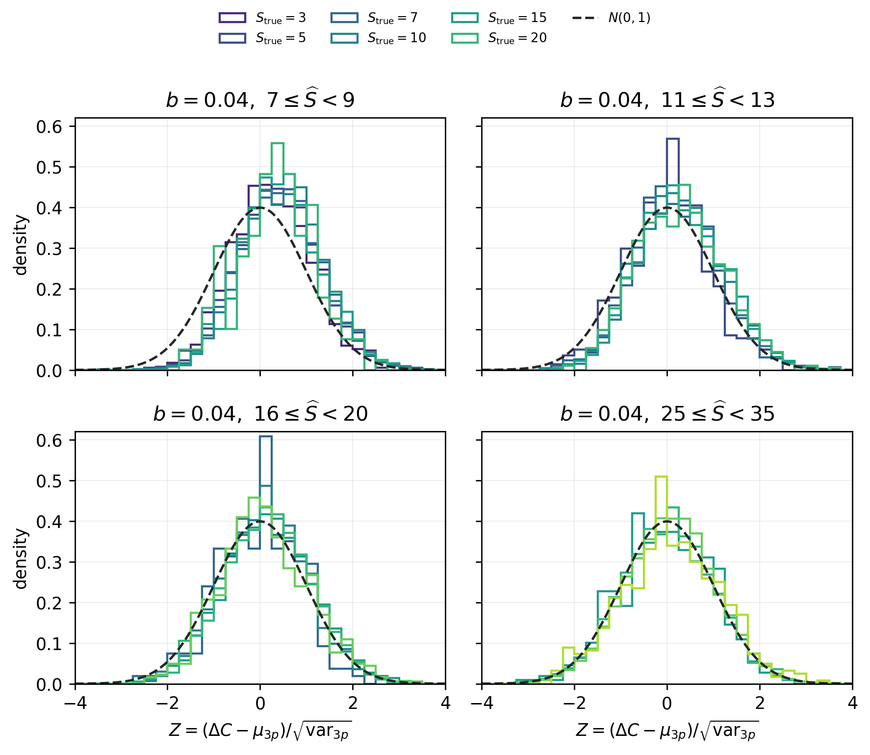
注入源强仅作诊断标签 条件理论仍按拟合振幅定义 / Injected source strength is only a diagnostic label while conditional theory uses fitted amplitude

Figure 2 is a diagnostic check on the conditioning variable. The simulations know the injected source strength $S_\mathrm{true}$, but the theory and the matched calibration condition on the fitted amplitude $\widehat{S}$. At fixed fitted $\widehat{S}$, the standardized residual distributions from different $S_\mathrm{true}$ subsets overlap closely. The residual offset in the lowest $\widehat{S}$ bin is the same low-signal beyond-Fisher bias discussed in Section 4.2, not evidence for conditioning on $S_\mathrm{true}$.

Acknowledgments

本研究使用了由 ESA 和 NASA 支持的 XMM Newton 数据 / This research used XMM Newton data supported by ESA and NASA

This research has made use of data obtained from the XMM-Newton satellite, an ESA science mission with instruments and contributions directly funded by ESA Member States and NASA.

References